![[ T∑ - t ]
n
max Et β u (ccct+n) ,
n=0](ctwMoM0x.png)
SED Version
_________________________________________________________________________________
Abstract
In a risky world, a pessimist assumes the worst will happen. Someone who
ignores risk altogether is an optimist. Consumption decisions are
mathematically simple for both the pessimist and the optimist because
both behave as if they live in a riskless world. A consumer who is
a realist (that is, who wants to respond optimally to risk) faces a
much more difficult problem, but (under standard conditions) will
choose a level of spending somewhere between that of the pessimist
and the optimist. We use this fact to redefine the space in which the
realist searches for optimal consumption rules. The resulting solution
accurately represents the numerical consumption rule over the entire
interval of feasible wealth values with remarkably few computations.
Dynamic Stochastic Optimization
FillInLater
| PDF: | http://www.econ2.jhu.edu/people/ccarroll/papers/ctwMoM.pdf |
| Slides: | http://www.econ2.jhu.edu/people/ccarroll/papers/ctwMoM-Slides.pdf |
| Web: | http://www.econ2.jhu.edu/people/ccarroll/papers/ctwMoM/ |
| Archive: | http://www.econ2.jhu.edu/people/ccarroll/papers/ctwMoM.zip |
1Carroll: Department of Economics, Johns Hopkins University, Baltimore, MD, http://www.econ2.jhu.edu/people/ccarroll/, ccarroll@jhu.edu 2Slacalek: European Central Bank, Frankfurt am Main, Germany, http://www.slacalek.com/, jiri.slacalek@ecb.europa.eu 3Tokuoka: International Monetary Fund, Washington, DC, ktokuoka@imf.org.
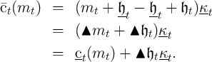
Solving a stochastic consumption, investment, portfolio choice, or similar continuous intertemporal optimization problem using numerical methods generally requires the modeler to choose how to represent a policy or value function. A common approach is to use low-order polynominal splines that exactly match the function (and maybe some derivatives) at each of a finite set of gridpoints, and then to assume that the matching polynomial is a good representation elsewhere.
This paper argues that, at least in the context of a standard consumption problem, there is a better approach, which relies upon the fact in the absence of uncertainty the optimal consumption function has a simple analytical solution. The key insight is that, under standard assumptions, the consumer who faces an uninsurable labor income risk will consume less (the consumer will engage in ‘precautionary saving’) than a consumer with the same path for expected income but who does not perceive any uncertainty as being attached to that future income. That is, the perfect foresight riskless solution provides an upper bound to the solution that will actually be optimal. A lower bound is provided by the behavior of a consumer who has the subjective belief that the future level of income will be the worst that it can possibly be. This consumer, too, behaves according to the analytical perfect foresight solution, but his certainty is that of an extremely overconfident pessimist.
Using results from Carroll (2011b), we show how to use these upper and lower bounds to tightly constrain the shape and characteristics of the solution to the ‘realist’s problem (that is, the solution to the problem of a consumer who correctly perceives the risks to future income and behaves rationally in response.
After showing how to use the method in the baseline case, we show how refine the method to encompass an even tighter theoretical bound, and how to extend it to solve a problem in which the consumer faces both labor income risk and rate-of-return risk.
|
| (1) |
It turns out (see Carroll (2011a) for a proof) that this problem can be
rewritten in a more convenient form in which choice and state variables are
normalized by the level of permanent income, e.g., using nonbold font for
normalized variables,  . When that is done, the transformed
version of the consumer’s problem is
. When that is done, the transformed
version of the consumer’s problem is
![v (m ) = max u(c ) + E [β Γ 1- ρv (m )] (7 )
t t ct t t t+1 t+1 t+1
s.t.
at = mt - ct
mt+1 = (R∕-Γ t+1-)at + θt+1
◟ ◝ ◜ ◞
≡Rt+1](ctwMoM5x.png)
For the remainder of the paper we will assume that permanent income  grows by a constant factor
  and is not subject to stochastic shocks. (The
generalization of the analysis below to the case of permanent shocks is
relatively straightforward.)
and is not subject to stochastic shocks. (The
generalization of the analysis below to the case of permanent shocks is
relatively straightforward.)
For comparison to our new solution method, we use the endogenous gridpoints
solution to the microeconomic problem presented in Carroll (2006). That
method computes the level of consumption at a set of gridpoints for market
resources  that are determined endogenously using the Euler equation.
The consumption function is then constructed by linear interpolation among
the gridpoints thus found.
that are determined endogenously using the Euler equation.
The consumption function is then constructed by linear interpolation among
the gridpoints thus found.
Carroll (2011a) describes a specific calibration of the model and constructs
a solution using five gridpoints chosen to capture the structure of
the consumption function reasonably well at values of  near the
infinite-horizon target value. (See those notes for details).
near the
infinite-horizon target value. (See those notes for details).
Unfortunately, the endogenous gridpoints solution is not very well-behaved
outside the original range of gridpoints targeted by the solution method.
(Though other common solution methods are no better outside their own
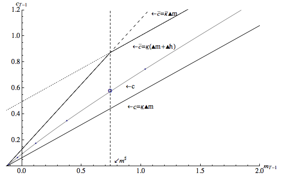
predefined ranges). Figure 1 demonstrates the point by plotting the
amount of precautionary saving implied by a linear extrapolation of our
approximated consumption rule (the consumption of the perfect foresight
consumer  minus our approximation to optimal consumption under
uncertainty,
minus our approximation to optimal consumption under
uncertainty,  ). Although theory proves that precautionary saving is
always positive, the linearly extrapolated numerical approximation
eventually predicts negative precautionary saving (at the point in the figure
where the extrapolated locus crosses the horizontal axis).
). Although theory proves that precautionary saving is
always positive, the linearly extrapolated numerical approximation
eventually predicts negative precautionary saving (at the point in the figure
where the extrapolated locus crosses the horizontal axis).
This problem cannot be solved by extending the upper gridpoint; in the presence of serious uncertainty, the consumption rule will need to be evaluated outside of any prespecified grid (because starting from the top gridpoint, a large enough realization of the uncertain variable will push next period’s realization of assets above that top). While a judicious extrapolation technique can prevent this problem from being fatal (for example by carefully excluding negative precautionary saving), the problem is often dealt with using inelegant methods whose implications for the accuracy of the solution are difficult to gauge.
As a preliminary to our solution, define  as end-of-period human wealth (the
present discounted value of future labor income) for a perfect foresight version of
the problem of a ‘risk optimist:’ a consumer who believes with perfect confidence
that the shocks will always take the value 1,
as end-of-period human wealth (the
present discounted value of future labor income) for a perfect foresight version of
the problem of a ‘risk optimist:’ a consumer who believes with perfect confidence
that the shocks will always take the value 1, ![θ = E [θ] = 1 ∀ n > 0
t+n](ctwMoM15x.png) .
The solution to a perfect foresight problem of this kind takes the
form2
.
The solution to a perfect foresight problem of this kind takes the
form2
 given below. We
similarly define
given below. We
similarly define  as ‘minimal human wealth,’ the present discounted value
of labor income if the shocks were to take on their worst possible value in
every future period
as ‘minimal human wealth,’ the present discounted value
of labor income if the shocks were to take on their worst possible value in
every future period 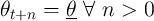 (which we define as corresponding to
the beliefs of a ‘pessimist’).
(which we define as corresponding to
the beliefs of a ‘pessimist’).
A first useful point is that, for the realist, a lower bound for the level of
market resources is  , because if
  equalled this value then there
would be a positive finite chance (however small) of receiving
equalled this value then there
would be a positive finite chance (however small) of receiving  in
every future period, which would require the consumer to set
in
every future period, which would require the consumer to set  to
zero in order to guarantee that the intertemporal budget constraint
holds. Since consumption of zero yields negative infinite utility, the
solution to realist consumer’s problem is not well defined for values
of
to
zero in order to guarantee that the intertemporal budget constraint
holds. Since consumption of zero yields negative infinite utility, the
solution to realist consumer’s problem is not well defined for values
of  , and the limiting value of the realist’s
  is zero as
 .
.
Given this result, it will be convenient to define ‘excess’ market resources as the amount by which actual resources exceed the lower bound, and ‘excess’ human wealth as the amount by which mean expected human wealth exceeds guaranteed minimum human wealth:
We can now transparently define the optimal consumption rules for the two
perfect foresight problems, those of the ‘optimist’ and the ‘pessimist.’ The
‘pessimist’ perceives human wealth to be equal to its minimum feasible value
 with certainty, so consumption is given by the perfect foresight solution
The ‘optimist,’ on the other hand, pretends that there is no uncertainty about future income, and therefore consumes
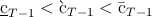
It seems obvious that the spending of the realist will be strictly greater
than that of the pessimist and strictly less than that of the optimist.
Figure 2 illustrates the proposition for the consumption rule in period
 .
.
Proof is more difficult than might be imagined, but the necessary work is done in Carroll (2011b) so we will take the proposition a fact and proceed by manipulating the inequality:
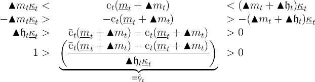
where the fraction in the middle of the last inequality is the ratio of
actual precautionary saving (the numerator is the difference between
perfect-foresight consumption and optimal consumption in the presence of
uncertainty) to the maximum conceivable amount of precautionary
saving (the amount that would be undertaken by the pessimist who
consumes nothing out of any future income beyond the perfectly
certain component). Defining  (which can range from
 to
to  ), the object in the middle of the last inequality is
 approaches
 .
.
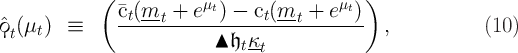
Given  , the consumption function can be recovered from
Thus, the procedure is to calculate  at the points
  corresponding to
the log of the
corresponding to
the log of the  points defined above, and then using these to construct
an interpolating approximation
points defined above, and then using these to construct
an interpolating approximation  from which we indirectly obtain our
approximated consumption rule
from which we indirectly obtain our
approximated consumption rule  by substituting
  for
for  in equation
(13).
in equation
(13).
Because this method relies upon the fact that the problem is easy to solve if the decision maker has unreasonable views (either in the optimistic or the pessimistic direction), and because the correct solution is always between these immoderate extremes, we call our solution procedure the ‘method of moderation.’
Results are shown in Figure 3; a reader with very good eyesight might be able to detect the barest hint of a discrepancy between the Truth and the Approximation at the far righthand edge of the figure.
Often it is useful to know the value function as well as the consumption rule associated with a problem. Fortunately, many of the tricks used when solving the consumption problem have a direct analogue in approximation of the value function.
Consider the perfect foresight (or ‘optimist’) case in period  :
:
 is the present discounted value of consumption. A similar
function can be constructed recursively for earlier periods, yielding the
general expression which can be transformed as
is the present discounted value of consumption. A similar
function can be constructed recursively for earlier periods, yielding the
general expression which can be transformed as 
 is a constant while the consumption function is linear,
  will also be linear.
We apply the same transformation to the value function for the problem with uncertainty (the realist’s problem):
 at the same gridpoints used by the
consumption function approximation, and interpolating among those
points.
at the same gridpoints used by the
consumption function approximation, and interpolating among those
points.
However, as with the consumption approximation, we can do even better if
we realize that the  function for the optimist’s problem is an upper bound
for the
function for the optimist’s problem is an upper bound
for the  function in the presence of uncertainty, and the value function for
the pessimist is a lower bound. Analogously to (10), define an upper-case
function in the presence of uncertainty, and the value function for
the pessimist is a lower bound. Analogously to (10), define an upper-case
 equation in (12):
and if we approximate these objects then invert them (as above with the
equation in (12):
and if we approximate these objects then invert them (as above with the  and
and  functions) we obtain a very high-quality approximation to our
inverted value function at the same points for which we have our
approximated value function:
functions) we obtain a very high-quality approximation to our
inverted value function at the same points for which we have our
approximated value function: 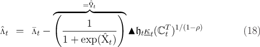
Although a linear interpolation that matches the level of  at the
gridpoints is simple, a Hermite interpolation that matches both the level and
the derivative of the
at the
gridpoints is simple, a Hermite interpolation that matches both the level and
the derivative of the  function at the gridpoints has the considerable
virtue that the
function at the gridpoints has the considerable
virtue that the  derived from it numerically satisfies the envelope
theorem at each of the gridpoints for which the problem has been
solved.
derived from it numerically satisfies the envelope
theorem at each of the gridpoints for which the problem has been
solved.
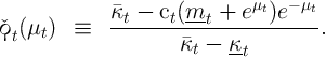
Carroll (2011b) derives an upper limit  for the MPC as
  approaches
its lower bound. Using this fact plus the strict concavity of the consumption
function yields the proposition that
approaches
its lower bound. Using this fact plus the strict concavity of the consumption
function yields the proposition that

The solution method described above does not guarantee that approximated consumption will respect this constraint between gridpoints, and a failure to respect the constraint can occasionally cause computational problems in solving or simulating the model. Here, we describe a method for constructing an approximation that always satisfies the constraint.
Defining  as the ‘cusp’ point where the two upper bounds intersect:
![mt ∈ (mt, m#t ]](ctwMoM79x.png) that respects
the tighter upper bound:
that respects
the tighter upper bound:
Again defining  , the object in the middle of the inequality is
 approaches
  ,
,  converges to zero, while as
  approaches
 ,
,  approaches
  .
.
As before, we can derive an approximated consumption function;
call it  . This function will clearly do a better job approximating
the consumption function for low values of
. This function will clearly do a better job approximating
the consumption function for low values of  while the previous
approximation will perform better for high values of
while the previous
approximation will perform better for high values of  .
.
For middling values of  it is not clear which of these functions will
perform better. However, an alternative is available which performs well.
Define the highest gridpoint below
it is not clear which of these functions will
perform better. However, an alternative is available which performs well.
Define the highest gridpoint below  as
as  and the lowest gridpoint
above
and the lowest gridpoint
above  as
as  . Then there will be a unique interpolating polynomial
that matches the level and slope of the consumption function at these two
points. Call this function
. Then there will be a unique interpolating polynomial
that matches the level and slope of the consumption function at these two
points. Call this function  .
.
Using indicator functions that are zero everywhere except for specified intervals,

To construct the corresponding refined representation of the value function we must first clarify one point: The upper-bound value function that we are constructing will be the one implied by a consumer whose spending behavior is consistent with the refined upper-bound consumption rule.
For  , this consumption rule is the same as before, so the
constructed upper-bound value function is also the same. However, for values
, this consumption rule is the same as before, so the
constructed upper-bound value function is also the same. However, for values
 matters are slightly more complicated.
Start with the fact that at the cusp point,
But for all  ,
,

 so for

 where
where  is as
defined above because a consumer who ends the current period with assets
exceeding the lower bound will not expect to be constrained next period.
(Recall again that we are merely constructing an object that is guaranteed to
be an upper bound for the value that the ‘realist’ consumer will experience.)
At the gridpoints defined by the solution of the consumption problem can
then construct
is as
defined above because a consumer who ends the current period with assets
exceeding the lower bound will not expect to be constrained next period.
(Recall again that we are merely constructing an object that is guaranteed to
be an upper bound for the value that the ‘realist’ consumer will experience.)
At the gridpoints defined by the solution of the consumption problem can
then construct 
 and
and  . The rest of
the procedure is analogous to that performed for the consumption rule and is
thus omitted for brevity.
. The rest of
the procedure is analogous to that performed for the consumption rule and is
thus omitted for brevity.
Thus far we have assumed that the interest factor is constant at  .
Extending the previous derivations to allow for a perfectly forecastable
time-varying interest factor
.
Extending the previous derivations to allow for a perfectly forecastable
time-varying interest factor  would be trivial. Allowing for a stochastic
interest factor is less trivial.
would be trivial. Allowing for a stochastic
interest factor is less trivial.

 is the long-run mean log interest factor,
  is the AR(1)
serial correlation coefficient, and
is the AR(1)
serial correlation coefficient, and  is the stochastic shock.
The consumer’s problem in this case now has two state variables,  and
and
 , and is described by
We approximate the AR(1) process by a Markov transition matrix using
standard techniques. The stochastic interest factor is allowed to take on 11
values centered around the steady-state value  and chosen [how?]. Given
this Markov transition matrix, conditional on the Markov AR(1) state the
consumption functions for the ‘optimist’ and the ‘pessimist’ will still be
linear, with identical MPC’s that are computed numerically. Given these
MPC’s, the (conditional) realist’s consumption function can be computed for
each Markov state, and the converged consumption rules constitute the
solution contingent on the dynamics of the stochastic interest rate
process.
and chosen [how?]. Given
this Markov transition matrix, conditional on the Markov AR(1) state the
consumption functions for the ‘optimist’ and the ‘pessimist’ will still be
linear, with identical MPC’s that are computed numerically. Given these
MPC’s, the (conditional) realist’s consumption function can be computed for
each Markov state, and the converged consumption rules constitute the
solution contingent on the dynamics of the stochastic interest rate
process.
In principle, this refinement should be combined with the previous one; further exposition of this combination is omitted here because no new insights spring from the combination of the two techniques.
The method proposed here is not universally applicable. For example, the method cannot be used for problems for which upper and lower bounds to the ‘true’ solution are not known. But many problems do have obvious upper and lower bounds, and in those cases (as in the consumption example used in the paper), the method may result in substantial improvements in accuracy and stability of solutions.
CARROLL, CHRISTOPHER D. (2006): “The Method of Endogenous Gridpoints for Solving Dynamic Stochastic Optimization Problems,” Economics Letters, pp. 312–320, http://www.econ2.jhu.edu/people/ccarroll/EndogenousGridpoints.pdf.
(2011a): “Solving Microeconomic Dynamic Stochastic Optimization Problems,” Archive, Johns Hopkins University.
(2011b): “Theoretical Foundations of Buffer Stock Saving,” Manuscript, Department of Economics, Johns Hopkins University, http://www.econ2.jhu.edu/people/ccarroll/papers/BufferStockTheory.
![′ - ρ ′
u (ct) = Et [βR Γ t+1u (ct+1)]. (8 )](ctwMoM6x.png)
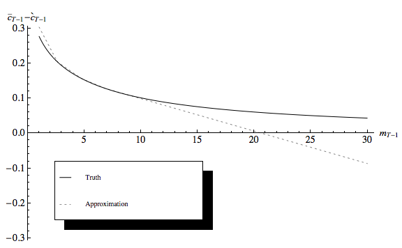
 , Predicted Precautionary Saving is Negative
(Oops!)
, Predicted Precautionary Saving is Negative
(Oops!)
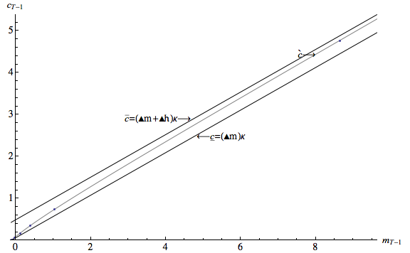

 Constructed Using the Method of Moderation

![( 1- ρ )1 ∕ρ
κ = 1 - β Et [R t+1 ] (22 )](ctwMoM117x.png)
![v(m ,r ) = max u(c ) + E [β Γ 1- ρv (m ,r )] (24 )
tt t ct t t t+1 t+1 t+1 t+1 t+1
s.t.
at = mt - ct
rt+1 - r = (rt - r)γ + ϵt+1
Rt+1 = exp (rt+1 )
m = (R ∕Γ ) a + θ .
t+1 ◟ --t+1◝◜--t+1◞ t t+1
≡Rt+1](ctwMoM124x.png)