Preliminary and Incomplete – Please Do Not
Quote
Digestible Microfoundations:
Buffer Stock Saving in a Krusell–Smith World
April 30, 2012
Christopher D. Carroll1
JHU
Jiri Slacalek2
ECB
Kiichi Tokuoka3
IMF
_____________________________________________________________________________________
Abstract
Krusell and Smith (1998) showed that it is possible to construct rational
expectations macroeconomic models with serious microfoundations. We argue
that three modifications to their framework are required to fulfill its promise.
First, we replace their assumption about household income dynamics with a
process that matches microeconomic data. Second, our agents have finite
lifetimes a la Blanchard (1985), which has both substantive and technical
benefits. Finally, we calibrate heterogeneity in time preference rates so
that the model matches the observed degree of inequality in the wealth
distribution. Our model has substantially different, and considerably more
plausible, implications for macroeconomic questions like the aggregate
marginal propensity to consume out of an economic ‘stimulus’ program.
-
Keywords
-
Microfoundations, Wealth Inequality, Marginal
Propensity to Consume
-
JEL codes
-
D12, D31, D91, E21
1Carroll: Department of Economics, Johns Hopkins University, Baltimore, MD,
http://www.econ2.jhu.edu/people/ccarroll/, ccarroll@jhu.edu 2Slacalek: European Central Bank,
Frankfurt am Main, Germany, http://www.slacalek.com/, jiri.slacalek@ecb.europa.eu 3Tokuoka:
International Monetary Fund, Washington, DC, ktokuoka@imf.org.
1 Introduction
Macroeconomists have sought credible microfoundations since the dawn of our
discipline. Keynes, his critics, and subsequent generations through Lucas (1976)
and beyond have agreed on this, if little else.
Since Keynes’s time, consumption modeling has been a battleground between
two microfoundational camps. ‘Bottom up’ modelers (e.g. Modigliani and
Brumberg (1954); Friedman (1957)) drew wisdom from microeconomic data and
argued that macro models should be constructed by aggregation from
microeconomic models that matched robust micro facts. ‘Top down’
modelers (e.g., Samuelson (1958); Diamond (1965); Hall (1978)) treated
aggregate consumption as reflecting the optimizing decisions of representative
agents; with only one such agent (or, at most, one per generation), these
models had ‘microfoundations’ under a generous interpretation of the
word.
The tractability of representative agent models has made them appealing for
business cycle analysis. But such models have never been easy to reconcile with either
macroeconomic
or microeconomic
evidence on consumption dynamics, nor with microeconomic theory which implies
that people who differ from each other (in age, preferences, wealth, liquidity
constraints, taxes, and other dimensions) should respond differently to any given
shock. If any of these differences matter (and it is hard to see how they could
not),
the aggregate size of a shock is not a sufficient statistic to calculate the
aggregate response; information about how the shock is distributed is
indispensable.
Bottom-up models, however, also have their problems. Even judged by a
sympathetic standard that asks how well they can match measured wealth
heterogeneity, bottom-up models have not been as successful as their champions
might have initially hoped. For example, bottom-up models calibrated to match
the wealth holdings of the median household generally fail to match the large
size of the aggregate capital stock, because they seriously underpredict the
upper parts of the wealth distribution (Carroll (2000b); Cagetti (2003)).
Alternatively, models calibrated to match the aggregate level of wealth greatly
overpredict wealth at the median (Hubbard, Skinner, and Zeldes (1994);
Carroll (2000b)). A further problem is that (at least until Krusell and
Smith (1998)) there has been no common answer to the question of how to
analyze systematic macroeconomic fluctuations (business cycles) in bottom-up
models.
This paper aims to reconcile the camps. We construct a workhorse
model that answers the main objections to both kinds of models by
making three modifications to the well-known Krusell–Smith (‘KS’)
framework.
First, we replace KS’s highly stylized assumptions about the nature of idiosyncratic
income shocks with a microeconomic labor income process that captures the
essentials of the empirical consensus from the labor economics literature about actual
income dynamics in micro data (with credibly calibrated transitory and permanent
shocks).
Second, agents in our model have finite lifetimes a la Blanchard (1985), permitting
a kind of primitive life cycle analysis and also solving some technical problems
created by the incorporation of permanent shocks. Finally, we obtain a necessary
extra boost to wealth inequality by calibrating a simple measure of heterogeneity in
‘impatience.’
The resulting framework differs sharply from the benchmark KS model in its
implications for important microeconomic and macroeconomic questions. A
timely macroeconomic example is the response of aggregate consumption to an
‘economic stimulus payment,’ interpreted here as a one-time lump sum transfer to
households. In response to a $1-per-capita payment, the baseline version of the KS
model implies that the annual marginal propensity to consume (MPC) is about
 ,
almost irrespective of how the cash is distributed across households. In contrast,
a version of our model that matches the distribution of liquid financial wealth
implies that if the entire tax cut were directed at households in the bottom half
of the liquid financial-wealth-to-income distribution, the MPC would be
,
almost irrespective of how the cash is distributed across households. In contrast,
a version of our model that matches the distribution of liquid financial wealth
implies that if the entire tax cut were directed at households in the bottom half
of the liquid financial-wealth-to-income distribution, the MPC would be
 , which counts as a big improvement in realism, given the vast
body of microeconomic evidence that consistently finds MPCs much
greater than the 3–5 percent figure that characterizes representative agent
models.
Furthermore, the model’s differences with the representative agent framework are
not peculiar to unusual events like a stimulus payment; to the extent that
different kinds of macroeconomic shocks tend systematically to be differently
distributed across the population (for example, labor income shocks may
affect a less wealthy set of households than capital income shocks), this
improvement in realism may also matter for general questions of macroeconomic
dynamics.
, which counts as a big improvement in realism, given the vast
body of microeconomic evidence that consistently finds MPCs much
greater than the 3–5 percent figure that characterizes representative agent
models.
Furthermore, the model’s differences with the representative agent framework are
not peculiar to unusual events like a stimulus payment; to the extent that
different kinds of macroeconomic shocks tend systematically to be differently
distributed across the population (for example, labor income shocks may
affect a less wealthy set of households than capital income shocks), this
improvement in realism may also matter for general questions of macroeconomic
dynamics.
Section 2 of the paper begins building the model’s structure by adding
microeconomic modeling elements to a benchmark representative agent model.
Using this model (without macroeconomic dynamics), the section closes by
estimating the degree of heterogeneity in impatience necessary to match the
degree of inequality in the U.S. wealth distribution; we find that relatively small
differences in impatience substantially affect the model’s fit to the wealth data.
Section 3 builds up the full version of the model by adding aggregate shocks of
the KS type, and presents detailed comparisons of our model with theirs.
Section 4 further improves the model by introducing an aggregate income
process that is analytically simpler than the KS ‘toy’ aggregate process, that we
believe is more empirically plausible as well, and that simplifies model
solution and simulation considerably. We offer this final, simpler version of
the model as our preferred jumping-off point for future macroeconomic
research.
2 The Model without Aggregate Uncertainty
2.1 The Perfect Foresight Representative Agent Model
To establish notation and a transparent benchmark, we begin by briefly
sketching a standard perfect foresight representative agent model.
The aggregate production function is
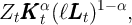 | (1) |
where  is aggregate productivity in period
  ,
,  is capital,
  is time
worked per employee, and
is time
worked per employee, and  is employment. The representative agent’s goal is
to maximize discounted utility from consumption
is employment. The representative agent’s goal is
to maximize discounted utility from consumption
for a CRRA utility function
 .
The representative agent’s state at the time of the consumption decision is
defined by two variables:
.
The representative agent’s state at the time of the consumption decision is
defined by two variables:  is market resources, and
  is aggregate
productivity.
is aggregate
productivity.
The transition process for  is broken up, for clarity of analysis and
consistency with later notation, into three steps. Assets at the end of the period
are market resources minus consumption, equal to
is broken up, for clarity of analysis and
consistency with later notation, into three steps. Assets at the end of the period
are market resources minus consumption, equal to
while next period’s capital is determined from this period’s assets via
The final step can be conceived as the transition from the beginning of period
 when capital has not yet been used to produce output, to the middle of
that period, when output has been produced and incorporated into resources but
has not yet been consumed:
when capital has not yet been used to produce output, to the middle of
that period, when output has been produced and incorporated into resources but
has not yet been consumed:
where  is the
interest rate,
is the
interest rate,  is the wage rate,
and
is the wage rate,
and  is the depreciation factor for capital.
After normalizing by the productivity factor
 ,
the representative agent’s problem is
,
the representative agent’s problem is
where the non-bold variables are the corresponding bold variables divided
by  (e.g.,
  ,
,  );
);  ; and the
expectations operator
; and the
expectations operator  here signifies the perfection of the agent’s foresight
(but will have the usual interpretation when uncertainty is introduced
below).
here signifies the perfection of the agent’s foresight
(but will have the usual interpretation when uncertainty is introduced
below).
Table 1: Parameter Values and Steady State
Notes: The models are calibrated at the quarterly frequency, and the steady state values are calculated on a
quarterly basis.
Except where otherwise noted, our parametric assumptions match
those of the papers in the special issue of the Journal of Economic
Dynamics and Control (2010, Volume 34, Issue 1, edited by den Haan,
Judd, and Julliard) devoted to comparing solution methods for the KS
model (the parameters are reproduced for convenience in the top panel of
Table 1).
The model is calibrated at the quarterly frequency. When aggregate shocks are
shut down ( and
and  ), the model has a steady-state solution with a
constant ratio of capital to output and constant (gross) interest and wage factors,
which we write without time subscript as
), the model has a steady-state solution with a
constant ratio of capital to output and constant (gross) interest and wage factors,
which we write without time subscript as  and
and  and which are reflected in
Table 1.
and which are reflected in
Table 1.
Henceforth, we refer to the version of the model solved by the papers in the
special JEDC volume as the ‘KS-JEDC’ model, while we call the original KS
model solved in Krusell and Smith (1998) ‘KS-Orig’ model. (The only effective
difference between the two is the introduction (for realism) of unemployment
insurance in the KS-JEDC version, which does not matter much for any substantive
results.  )
)
2.2 The Household Income Process
For our purposes, the principal conclusion of the large literature on microeconomic
labor income dynamics is that household income can be reasonably well
described as follows. The idiosyncratic permanent component of labor income  evolves according to
where  captures the predictable low-frequency (e.g., life-cycle and
demographic) components of income growth, and the Greek letter psi
mnemonically indicates the permanent shock to income. Actual income is the
product of permanent income, a mean-one transitory shock, and the wage
rate:
captures the predictable low-frequency (e.g., life-cycle and
demographic) components of income growth, and the Greek letter psi
mnemonically indicates the permanent shock to income. Actual income is the
product of permanent income, a mean-one transitory shock, and the wage
rate:
After taking logarithms, this income process is strikingly similar to
Friedman (1957)’s characterization of income as having permanent and transitory
components. Because this process has been used widely in the literature on
buffer stock saving, and though similar to Friedman’s formulation is not identical
to it, we henceforth refer to it as the Friedman/Buffer Stock (or ‘FBS’)
process.
Table 2 summarizes the annual variances of log permanent shocks ( ) and
log transitory shocks (
) and
log transitory shocks ( ) estimated by a selection of papers from the extensive
literature.
Some authors have used a process of this kind to describe the labor income or
wage process for an individual worker (top panel) while others have used it to
describe the process for overall household income (bottom panel); it seems to
work reasonably well in both cases (though, obviously, with different estimates of
the variances). (Recent work by Sabelhaus and Song (2010) using newly
available data from Social Security earnings files finds that the variances of both
transitory and permanent shocks have declined during the “Great Moderation”
period at all ages; they also find distinct life cycle patterns of shocks by age, with
young people experiencing higher levels of both kinds of shocks than the
middle-aged).
) estimated by a selection of papers from the extensive
literature.
Some authors have used a process of this kind to describe the labor income or
wage process for an individual worker (top panel) while others have used it to
describe the process for overall household income (bottom panel); it seems to
work reasonably well in both cases (though, obviously, with different estimates of
the variances). (Recent work by Sabelhaus and Song (2010) using newly
available data from Social Security earnings files finds that the variances of both
transitory and permanent shocks have declined during the “Great Moderation”
period at all ages; they also find distinct life cycle patterns of shocks by age, with
young people experiencing higher levels of both kinds of shocks than the
middle-aged).
The second-to-last line of the table shows what labor economists would have found,
when estimating a process like the one above, if the empirical data were generated by
households who experienced an income process like the one assumed by the KS-JEDC
model.
This row of the table makes our point forcefully: The empirical procedures that
have actually been applied to empirical micro data, if used to measure the
income process households experience in a KS economy, would have
produced estimates of  and
and  that are orders of magnitude
different from what the actual empirical literature finds in actual data.
This discrepancy naturally makes one wonder whether the KS-JEDC
model’s well-known difficulty in matching the degree of wealth inequality is
largely explained by its highly unrealistic assumption about the income
process.
that are orders of magnitude
different from what the actual empirical literature finds in actual data.
This discrepancy naturally makes one wonder whether the KS-JEDC
model’s well-known difficulty in matching the degree of wealth inequality is
largely explained by its highly unrealistic assumption about the income
process.
Table 2: Estimates of Annual Variances of Log Income, Earning and Wage Shocks
Notes:  MaCurdy (1982) did not explicitly separate
  and
and  , but we have extracted
  and
and  as
implications of statistics that his paper reports. First, we calculate
as
implications of statistics that his paper reports. First, we calculate  and
and
 using his estimate (we set
  ). Then, following Carroll and Samwick (1997) we
obtain the values of
). Then, following Carroll and Samwick (1997) we
obtain the values of  and
and  which can match these statistics, assuming that the income
process is
which can match these statistics, assuming that the income
process is  and
and  (i.e., we solve
  and
and
 ).
).  Moffitt and Gottschalk (1995) estimated the income process
with random walk plus ARMA. Using income draws generated by their estimated process and following Carroll
and Samwick (1997), we have estimated the variances under the assumption that these income draws were
produced by the process
Moffitt and Gottschalk (1995) estimated the income process
with random walk plus ARMA. Using income draws generated by their estimated process and following Carroll
and Samwick (1997), we have estimated the variances under the assumption that these income draws were
produced by the process  where
where  .
.  Meghir and Pistaferri (2004), Jensen and
Shore (2008), Hryshko (2010), and Blundell, Pistaferri, and Preston (2008) assume that the transitory
component is serially correlated (an MA process), and report the variance of a subelement of the transitory
component. For example, Meghir and Pistaferri (2004) and Blundell, Pistaferri, and Preston (2008) assume
an MA(1) process
Meghir and Pistaferri (2004), Jensen and
Shore (2008), Hryshko (2010), and Blundell, Pistaferri, and Preston (2008) assume that the transitory
component is serially correlated (an MA process), and report the variance of a subelement of the transitory
component. For example, Meghir and Pistaferri (2004) and Blundell, Pistaferri, and Preston (2008) assume
an MA(1) process  and obtain estimates
  =
= and
and
 , respectively.
  for these four articles reported in this table are calculated by
 using their estimates.
2.3 Finite Lifetimes and the Finite Variance of Permanent Income in the
Cross-Section
One might wish to use the FBS income process specified in subsection
2.2 as a complete characterization of household income dynamics, but
that idea has a problem: Since each household accumulates a permanent
shock in every period, the cross-sectional distribution of idiosyncratic
permanent income becomes wider and wider indefinitely as the simulation
progresses; that is, there is no ergodic distribution of permanent income in the
population.
This problem and several others can be addressed by assuming that the
model’s agents have finite lifetimes a la Blanchard (1985). Death follows a
Poisson process, so that every agent alive at date  has an equal probability
  of dying before the beginning of period
  . (The probability of NOT dying is
the cancelation of the probability of dying:
. (The probability of NOT dying is
the cancelation of the probability of dying:  ). Households engage in a
Blanchardian mutual insurance scheme: Survivors share the estates of those who
die. Assuming a zero profit condition for the insurance industry, the
insurance scheme’s ultimate effect is simply to boost the rate of return
(for survivors) by an amount exactly corresponding to the mortality
rate.
). Households engage in a
Blanchardian mutual insurance scheme: Survivors share the estates of those who
die. Assuming a zero profit condition for the insurance industry, the
insurance scheme’s ultimate effect is simply to boost the rate of return
(for survivors) by an amount exactly corresponding to the mortality
rate.
In order to maintain a constant population (of mass one, uniformly distributed
on the unit interval), we assume that dying households are replaced by an
equal number of newborns; we write the population-mean operator as
![∫ 1
M [∙t] = 0 ∙t,ιdι](BSinKS85x.png) . Newborns, we assume, begin life with a level of idiosyncratic
permanent income equal to the mean level of idiosyncratic permanent income in
the population as a whole. Conveniently, our definition of the permanent shock
implies that in a large population, mean idiosyncratic permanent income
will remain fixed at
. Newborns, we assume, begin life with a level of idiosyncratic
permanent income equal to the mean level of idiosyncratic permanent income in
the population as a whole. Conveniently, our definition of the permanent shock
implies that in a large population, mean idiosyncratic permanent income
will remain fixed at ![M [p] = 1](BSinKS86x.png) forever, while the mean of
forever, while the mean of  is given
by
is given
by
and
the variance of  by
by
Of course for all of this to be valid, it is necessary to impose the parametric
restriction ![/ 2
/D E [ψ ] < 1](BSinKS91x.png) (a requirement that does not do violence to the data, as
we shall see). Intuitively, the requirement is that, among surviving consumers,
income does not spread out so quickly as to overwhelm the compression of the
permanent income distribution that arises because of the equalizing force of
death and replacement.
(a requirement that does not do violence to the data, as
we shall see). Intuitively, the requirement is that, among surviving consumers,
income does not spread out so quickly as to overwhelm the compression of the
permanent income distribution that arises because of the equalizing force of
death and replacement.
Since our goal here is to produce a realistic distribution of permanent
income across the members of the (simulated) population, we measure the
empirical distribution of permanent income in the cross section using
data from the Survey of Consumer Finances (SCF), which conveniently
includes a question asking respondents whether their income in the survey
year was about ‘normal’ for them, and if not, asks the level of ‘normal’
income.
This corresponds well with our (and Friedman (1957)’s) definition of permanent
income  (and Kennickell (1995) shows that the answers people give to this
question can be reasonably interpreted as reflecting their perceptions of their
permanent income), so we calculate the variance of
(and Kennickell (1995) shows that the answers people give to this
question can be reasonably interpreted as reflecting their perceptions of their
permanent income), so we calculate the variance of ![i i i
p ≡ p ∕M [p ]](BSinKS93x.png) among such
households.
among such
households.
The results from this exercise are reported in Table 3 (with a final
row that makes the point that both the KS-Orig and KS-JEDC models
assume that permanent shocks did not exist). Substituting these estimates
for  into (7) and (8), we obtain estimates of the variance of
  .
Reassuringly, we can interpret the variances of
.
Reassuringly, we can interpret the variances of  thus obtained as
being easily in the range of the estimated variances of
thus obtained as
being easily in the range of the estimated variances of  in
Table 2.
Such a correspondence, across two quite different methods of measurement,
suggests there is considerable robustness to the measurement of the size of
permanent shocks. (Below, we will choose a calibration for
in
Table 2.
Such a correspondence, across two quite different methods of measurement,
suggests there is considerable robustness to the measurement of the size of
permanent shocks. (Below, we will choose a calibration for  that is in the
middle range of estimates from either method.)
that is in the
middle range of estimates from either method.)
Table 3: Variance of Permanent Income
2.4 The Wealth Distribution with Transitory and Permanent Shocks
We now examine how wealth would be distributed in the steady-state
equilibrium of an economy with wage rates and interest rates fixed at the
steady state values calibrated in Table 1 of subsection 2.1, an income
process like the one described in subsection 2.2, and finite lifetimes per
subsection 2.3.
The process of noncapital income of each household follows
where  is noncapital income for the household in period
  , equal to
the permanent component of noncapital income
, equal to
the permanent component of noncapital income  multiplied by a
transitory income shock factor
multiplied by a
transitory income shock factor  and wage rate
  ; the permanent
component of noncapital income in period
; the permanent
component of noncapital income in period  is equal to its previous value,
multiplied by a mean-one iid shock
is equal to its previous value,
multiplied by a mean-one iid shock  ,
, ![E [ψ ] = 1
t t+n](BSinKS108x.png) for all
for all  .
.
 is capital and
  is the employment rate (because
  is
the unemployment rate). Since there is no aggregate shock,
is
the unemployment rate). Since there is no aggregate shock,  ,
,  ,
,
 , and
, and  are constant (
 ,
,  ,
,  , and
, and
 ).
).
Following the assumptions in the JEDC volume, the distribution of  is:
is:
where
 is the unemployment insurance payment when unemployed and
  is the rate of tax collected to pay unemployment benefits (see Table 1 for parameter
values).
The probability of unemployment is constant (
is the rate of tax collected to pay unemployment benefits (see Table 1 for parameter
values).
The probability of unemployment is constant ( ); later we allow
  to
vary over time.
to
vary over time.
The decision problem for the household in period  can be written using
normalized variables; the consumer’s objective is to choose a series of
consumption functions
can be written using
normalized variables; the consumer’s objective is to choose a series of
consumption functions  between now and the end of the horizon that satisfy:
where the non-bold ratio variables are defined as the bold (level) variables
divided by the level of permanent income  (e.g.,
  ).
The only state variable is (normalized) cash-on-hand
).
The only state variable is (normalized) cash-on-hand  . The household’s
employment status is not a state variable, unlike in the KS-JEDC model, where
tomorrow’s employment status depends on today’s status. This substantially
simplifies the analysis (which is useful for computational and analytical
purposes), arguably without too much sacrifice of realism (except possibly for
detailed studies of the behavior of households during extended unemployment
spells).
. The household’s
employment status is not a state variable, unlike in the KS-JEDC model, where
tomorrow’s employment status depends on today’s status. This substantially
simplifies the analysis (which is useful for computational and analytical
purposes), arguably without too much sacrifice of realism (except possibly for
detailed studies of the behavior of households during extended unemployment
spells).
Since households die with a constant probability  between periods, the effective
discount factor is
between periods, the effective
discount factor is  (in (13)); the effective interest rate is
  (combining (14)
and (15)).
(combining (14)
and (15)).
Aside from heterogeneity in impatience (introduced below), three parameters
characterize our modifications to the KS-JEDC model:  ,
,  , and
, and  .
.
 implies the average length of working life is
  quarters
=
quarters
=  years (dating from entry into the labor force at, say, age 25). The
variance of log transitory income shocks
years (dating from entry into the labor force at, say, age 25). The
variance of log transitory income shocks  is the value advocated in
Carroll (1992) (based on the Panel Study of Income Dynamics (PSID)
data),
as is
is the value advocated in
Carroll (1992) (based on the Panel Study of Income Dynamics (PSID)
data),
as is  (but note that this value also matches the median value in
Table 3).
(but note that this value also matches the median value in
Table 3).  Other parameter values (
 ,
,  ,
,  , and
, and  ) are from the JEDC volume
(Table 1).
) are from the JEDC volume
(Table 1).
The one remaining unspecified parameter is the time preference factor.
As a preliminary theoretical consideration, note that Carroll (2011)
(generalizing Deaton (1991) and Bewley (1977)) has shown that models of
this kind do not have a well-defined solution unless the condition holds:
where
Carroll (2011) dubs this inequality the ‘Growth Impatience Condition’ because
it guarantees that consumers are sufficiently impatient to prevent the indefinite
increase in the ratio of net worth to permanent income when income is growing
(see also Szeidl (2006)). This condition is an amalgam of the pure time
preference factor, expected growth, the relative risk aversion coefficient,
and the real interest factor. Thus, a consumer can be ‘impatient’ in the
required sense even if  , so long as expected income growth is
positive.
, so long as expected income growth is
positive.
We begin by searching for the time preference factor  such that if all households
had an identical
such that if all households
had an identical  the steady-state value of the capital-to-output ratio (
 )
would match the value that characterized the steady-state of the perfect foresight
model.
)
would match the value that characterized the steady-state of the perfect foresight
model.
 turns out to be
  (recall that this is at a quarterly, not an annual,
rate).
(recall that this is at a quarterly, not an annual,
rate).
We now ask whether this model with realistically calibrated income and finite
lifetimes (henceforth, the model is referred to as the ‘ -Point’ model) can
reproduce the degree of wealth inequality evident in the micro data. An
improvement in the model’s ability to match the data is to be expected, since in
buffer stock models agents strive to achieve a target ratio of wealth to permanent
income. By assuming no dispersion in the level of permanent income across
households, KS’s income process disables a potentially vital explanation for
variation in the level of target wealth (and, therefore, on average, actual wealth)
across households.
-Point’ model) can
reproduce the degree of wealth inequality evident in the micro data. An
improvement in the model’s ability to match the data is to be expected, since in
buffer stock models agents strive to achieve a target ratio of wealth to permanent
income. By assuming no dispersion in the level of permanent income across
households, KS’s income process disables a potentially vital explanation for
variation in the level of target wealth (and, therefore, on average, actual wealth)
across households.
Table 4: Proportion of Net Worth by Percentile (in percent)
Table 4 shows that compared to the distribution of net worth
implied by our solution of the KS-JEDC model solved without an
aggregate shock (or the results of the KS-Orig model from Krusell and
Smith (1998)),
our  -Point model does indeed yield a substantial improvement
(compare the first, third and fourth columns to the last
column).
For example, in our
-Point model does indeed yield a substantial improvement
(compare the first, third and fourth columns to the last
column).
For example, in our  -Point model, the fraction of total net worth held by the
top 1 percent is about 10 percent, while the corresponding statistic is
only 3 percent in our solution of the KS-JEDC model (or the KS-Orig
model).
-Point model, the fraction of total net worth held by the
top 1 percent is about 10 percent, while the corresponding statistic is
only 3 percent in our solution of the KS-JEDC model (or the KS-Orig
model).
The KS-JEDC model’s failure to match the wealth distribution is not confined
to the top. In fact, perhaps a bigger problem is that the model generates a
distribution of wealth in which most households’ wealth levels are not very far
from the wealth target of a representative agent in the perfect foresight
version of the model. For example, in steady state about  percent
of all households in the KS-JEDC model have net worth between 0.5
times mean net worth and 1.5 times mean net worth; in the SCF data
from 1992–2004, the corresponding fraction ranges from only 20 to 25
percent.
percent
of all households in the KS-JEDC model have net worth between 0.5
times mean net worth and 1.5 times mean net worth; in the SCF data
from 1992–2004, the corresponding fraction ranges from only 20 to 25
percent.
But while the  -Point model fits the data better than the original KS model,
it still falls short of matching the empirical degree of wealth inequality. The
proportion of net worth held by households in the top 1 percent of the
distribution is three times smaller in the model than in the data (compare the
first and last columns in the table). This failure reflects the fact that, empirically,
the distribution of wealth is considerably more unequal than the distribution of
permanent income.
-Point model fits the data better than the original KS model,
it still falls short of matching the empirical degree of wealth inequality. The
proportion of net worth held by households in the top 1 percent of the
distribution is three times smaller in the model than in the data (compare the
first and last columns in the table). This failure reflects the fact that, empirically,
the distribution of wealth is considerably more unequal than the distribution of
permanent income.
2.5 Heterogeneous Impatience
As the simplest method to address this defect, we introduce heterogeneity in impatience:
Each household is now assumed to have an idiosyncratic (but fixed) time preference
factor.
We do not think of this assumption as only capturing actual variation in pure
rates of time preference across people (though such variation surely exists).
Instead, we view discount-factor heterogeneity as a shortcut that captures the
essential consequences of many other kinds of heterogeneity (e.g., heterogeneity
in age, income growth expectations, investment opportunities, tax schedules) as
well. To be more concrete, take the example of age. A robust pattern in most
countries is that income grows much faster for young people than for older
people. According to (16), young people should therefore tend to act, financially,
in a more ‘impatient’ fashion than older people. In particular, we should expect
them to have lower target wealth-to-income ratios. Thus, what we are
capturing by allowing heterogeneity in time preference factors is probably
also some portion of the difference in behavior that (in truth) reflects
differences in age instead of in time preference factors, and that would be
introduced into the model if we had a more complex specification of the life
cycle that allowed for different growth rates for households of different
ages.
One way of gauging a model’s predictions for wealth inequality is to ask how
well it is able to match the proportion of total net worth held by the
wealthiest  ,
,  ,
,  , and
, and  percent of the population. Because
these statistics have been targeted by other papers (e.g., Castaneda,
Diaz-Gimenez, and Rios-Rull (2003)), we adopt a goal of matching
them.
percent of the population. Because
these statistics have been targeted by other papers (e.g., Castaneda,
Diaz-Gimenez, and Rios-Rull (2003)), we adopt a goal of matching
them.
We replace the assumption that all households have the same time
preference factor with an assumption that, for some  , time preference
factors are distributed uniformly in the population between
, time preference
factors are distributed uniformly in the population between  and
and
 (for this reason, the model is referred to as the ‘
 -Dist’ model
below). Then, using simulations, we search for the values of
-Dist’ model
below). Then, using simulations, we search for the values of  and
and
 for which the model best matches the fraction of net worth held
by the top
for which the model best matches the fraction of net worth held
by the top  ,
,  ,
,  , and
, and  percent of the population, while
at the same time matching the aggregate capital-to-output ratio from
the perfect foresight model. Specifically, defining
percent of the population, while
at the same time matching the aggregate capital-to-output ratio from
the perfect foresight model. Specifically, defining  and
and  as the
proportion of total aggregate net worth held by the top
as the
proportion of total aggregate net worth held by the top  percent in our
model and in the data, respectively, we solve the following minimization
problem:
percent in our
model and in the data, respectively, we solve the following minimization
problem:
 | (17) |
subject to the constraint that the aggregate wealth (net worth)-to-output ratio in the
model matches the aggregate capital-to-output ratio from the perfect foresight model
( ):
):
The
solution to this problem is  .
.
The introduction of even such a relatively modest amount of time preference
heterogeneity sharply improves the model’s fit to the targeted proportions of
wealth holdings (second column of the table). The ability of the model to match
the targeted moments does not, of course, constitute a formal test, except in the
loose sense that a model with such strong structure might have been unable
to get nearly so close to four target wealth points with only one free
parameter.
But the model also sharply improves the fit to locations in the wealth
distribution that were not explicitly targeted; for example, the net worth shares
of the top 10 percent and the top 1 percent are also included in the table, and
the model performs reasonably well in matching them.
Of course, Krusell and Smith (1998) were well aware that their baseline model
match the wealth distribution well. They, too, examined whether inclusion of a
form of discount rate heterogeneity could improve the model’s match to
the data. Specifically, they assumed that the discount factor takes one
of the three values ( ,
,  , and
, and  ), and that agents
anticipate that their discount factor might change between these values
according to a Markov process. As they showed, the model with this
simple form of heterogeneity (henceforth ‘KS-Orig Hetero’ model) did
improve the model’s ability to match the wealth holdings of the top
percentiles (see KS-Orig Hetero column in the table). Indeed, as inspection of
the long-dashing locus in Figure 1 shows, their model of heterogeneity
went a bit too far: It concentrated almost all of the net worth in the
top 20 percent of the population (though rather evenly among that top
20 percent). By comparison, the figure shows that our model does a
notably better job matching the data across the entire span of wealth
percentiles.
), and that agents
anticipate that their discount factor might change between these values
according to a Markov process. As they showed, the model with this
simple form of heterogeneity (henceforth ‘KS-Orig Hetero’ model) did
improve the model’s ability to match the wealth holdings of the top
percentiles (see KS-Orig Hetero column in the table). Indeed, as inspection of
the long-dashing locus in Figure 1 shows, their model of heterogeneity
went a bit too far: It concentrated almost all of the net worth in the
top 20 percent of the population (though rather evenly among that top
20 percent). By comparison, the figure shows that our model does a
notably better job matching the data across the entire span of wealth
percentiles.
The reader might wonder why we do not simply adopt the KS specification of
heterogeneity in time preference factors, rather than introducing our own novel
form of heterogeneity. The principal answer is that our purpose here is to define
a method of explicitly matching the model to the data via statistical estimation
of a parameter of the distribution of heterogeneity, letting the data speak flexibly
to the question of the extent of the heterogeneity required to match model to
data. A second point is that, having introduced finite horizons in order to yield
an ergodic distribution of permanent income, it would be peculiar to layer
on top of the stochastic death probability a stochastic probability of
changing one’s time preference factor within the lifetime; Krusell and Smith
motivated their differing time preference factors as reflecting different
preferences of alternative generations of a dynasty, but with our finite
horizons assumption we have eliminated the dynastic interpretation of the
model. Having said all of this, the common point across the two papers
is that a key requirement to make the model fit the data is a form of
heterogeneity that leads different households to have different target levels of
wealth.
3 KS Aggregate Shocks
In this section, we examine a model with an FBS household income process
that also incorporates KS aggregate shocks, and investigate the model’s
performance in replicating aggregate statistics. Krusell and Smith (1998)
assumed that the level of aggregate productivity alternates between
 if the aggregate state is good and
  if it is bad;
similarly,
if it is bad;
similarly,  where
where  if the state is good and
  if
bad. (For reference, we reproduce their assumed parameter values in
Table 5.)
if
bad. (For reference, we reproduce their assumed parameter values in
Table 5.)
Table 5: Parameter Values for Aggregate Shocks
The decision problem for an individual household in period  can be written
using normalized variables and the employment status
can be written
using normalized variables and the employment status  :
:
where
- the non-bold individual variables (lower-case variables except for
 and
and  ) are the bold (level) variables divided by
  (e.g.,
 ,
,  ),
),
 ,
,
 , and
, and
- the income process is the same as in (8)–(12) but the employment
transition process follows KS-JEDC.
There are more state variables in this version of the model than in the model
with no aggregate shock: The aggregate variables  and
and  , and the
household’s employment status
, and the
household’s employment status  whose transition process depends on the
aggregate state. Solving the full version of the model above with both aggregate
and idiosyncratic shocks is not straightforward; the basic idea for the solution
method is the key insight of Krusell and Smith (1998). See Appendix C for
details about our solution method.
whose transition process depends on the
aggregate state. Solving the full version of the model above with both aggregate
and idiosyncratic shocks is not straightforward; the basic idea for the solution
method is the key insight of Krusell and Smith (1998). See Appendix C for
details about our solution method.
We now report the results of simulations, both for the model in which all
households have the same time preference factor ( -Point model) and for the
version with a uniform distribution of time preference factors (
-Point model) and for the
version with a uniform distribution of time preference factors ( -Dist model).
While the
-Dist model).
While the  -Point model uses
  estimated in Section 2, the
  -Dist model
uses parameter values reestimated by solving the minimization problem (17)
with the KS aggregate shocks (
-Dist model
uses parameter values reestimated by solving the minimization problem (17)
with the KS aggregate shocks ( ). Results using
our solution of the KS-JEDC model (with the KS aggregate shocks,
). Results using
our solution of the KS-JEDC model (with the KS aggregate shocks,
 ,
,  for all
  , and no death (
 )) are also reported for
comparison.
)) are also reported for
comparison.
3.1 Some Macroeconomic Statistics
Table 6 shows some aggregate statistics that we think are useful for macroeconomic
analysis: The serial correlation of consumption growth, and correlation between
consumption growth, income growth, and interest rates at several frequencies.
The results are generally similar across the  -Point,
  -Dist, and KS-JEDC
models. They all produce positive
-Dist, and KS-JEDC
models. They all produce positive  , and high correlation
of consumption growth with (current) income growth or (current) interest rates.
The serial correlation of consumption growth in our solution of the
KS-JEDC model is similar to that reported by Maliar, Maliar, and
Valli (2008) who also solved the KS-JEDC model (fourth column of the
table).
, and high correlation
of consumption growth with (current) income growth or (current) interest rates.
The serial correlation of consumption growth in our solution of the
KS-JEDC model is similar to that reported by Maliar, Maliar, and
Valli (2008) who also solved the KS-JEDC model (fourth column of the
table).  We also report results for the representative agent model with the KS aggregate
income shock parameters (last column), the results of which are very close to
those of our solution of the KS-JEDC model.
We also report results for the representative agent model with the KS aggregate
income shock parameters (last column), the results of which are very close to
those of our solution of the KS-JEDC model.
Table 6: Aggregate Statistics with KS Aggregate Shocks
Notes:  and
and  are one-year and two-year growth rates, respectively.
The classic reference point for consumption growth measurement is the
random walk model of Hall (1978), and the large literature that rejects the
random walk proposition in favor of models that either contain some
‘rule-of-thumb’ consumers who set spending equal to income in every period
(Campbell and Mankiw (1989)) or, more popular recently, models with habit
formation or ‘sticky expectations’ (Carroll, Slacalek, and Tokuoka (2008)) that
imply serial correlation in consumption growth (see Carroll, Sommer, and
Slacalek (2011) for evidence).
The KS-JEDC model produces a relatively high correlation coefficient
 , which is closer to the U.S. data (where the statistic is about
one-third) than that produced by standard consumption models stemming from
Hall (1978).
As noted already, our
, which is closer to the U.S. data (where the statistic is about
one-third) than that produced by standard consumption models stemming from
Hall (1978).
As noted already, our  -Point and
  -Dist models also imply positive
 , although not as high as that predicted by the
KS-JEDC model. At first blush, it seems puzzling that the KS-JEDC model,
which includes neither habits nor sticky expectations, generates a substantial
violation of the random walk proposition. This puzzle does not seem to have
been noticed in the previous literature on the KS-JEDC model, but after
some investigation we determined that the KS-JEDC model’s sticky
consumption growth is produced by the high degree of serial correlation in
interest rates in the model, which results from the assumption about the
process of aggregate productivity shocks (see Appendix D for details). The
interesting questions, in a model with time-varying interest rates, are,
first, whether one can reliably estimate an intertemporal elasticity of
substitution (IES) from the coefficient in a regression of consumption on the
predictable component of interest rates (as Hall (1988) attempts to do),
and, second, whether consumption growth is serially correlated after
accounting for the predictable component related to interest rates (no random
walk).
, although not as high as that predicted by the
KS-JEDC model. At first blush, it seems puzzling that the KS-JEDC model,
which includes neither habits nor sticky expectations, generates a substantial
violation of the random walk proposition. This puzzle does not seem to have
been noticed in the previous literature on the KS-JEDC model, but after
some investigation we determined that the KS-JEDC model’s sticky
consumption growth is produced by the high degree of serial correlation in
interest rates in the model, which results from the assumption about the
process of aggregate productivity shocks (see Appendix D for details). The
interesting questions, in a model with time-varying interest rates, are,
first, whether one can reliably estimate an intertemporal elasticity of
substitution (IES) from the coefficient in a regression of consumption on the
predictable component of interest rates (as Hall (1988) attempts to do),
and, second, whether consumption growth is serially correlated after
accounting for the predictable component related to interest rates (no random
walk).
3.2 The Aggregate Marginal Propensity to Consume
A macroeconomic question of perhaps even greater interest is whether a
model that manages to match the distribution of wealth has similar, or
different, implications from the KS-JEDC or representative agent models
for the reaction of aggregate consumption to an economic ‘stimulus’
payment.
Specifically, we pose the question as follows. The economy has been in its
steady-state equilibrium leading up to date  . Before the consumption decision
is made in that period, the government announces the following plan: Effective
immediately, every household in the economy will receive a ‘stimulus check’
worth some modest amount $
. Before the consumption decision
is made in that period, the government announces the following plan: Effective
immediately, every household in the economy will receive a ‘stimulus check’
worth some modest amount $ (financed by a tax on unborn future
generations).
(financed by a tax on unborn future
generations).
In theory, the distribution of wealth across recipients of the stimulus checks has
important implications for aggregate MPC out of transitory shocks to income.
To see why, the solid line of Figure 2 plots our  -Point model’s individual
consumption function in the good (aggregate) state, with the horizontal axis
being cash on hand normalized by the level of (quarterly) permanent
income. Because the households with less normalized cash have higher
MPC,
the average MPC is higher when a larger fraction of households has less
(normalized) cash on hand.
-Point model’s individual
consumption function in the good (aggregate) state, with the horizontal axis
being cash on hand normalized by the level of (quarterly) permanent
income. Because the households with less normalized cash have higher
MPC,
the average MPC is higher when a larger fraction of households has less
(normalized) cash on hand.
There are many more households with little wealth in our  -Point model
than in the KS-JEDC model, as illustrated by comparison of the short-dashing
and the long-dashing lines in Figure 1. The greater concentration of wealth at
the bottom in the
-Point model
than in the KS-JEDC model, as illustrated by comparison of the short-dashing
and the long-dashing lines in Figure 1. The greater concentration of wealth at
the bottom in the  -Point model, which is the case in the data (see the
histogram in Figure 2), should produce a higher average MPC, given the
concave consumption function.
-Point model, which is the case in the data (see the
histogram in Figure 2), should produce a higher average MPC, given the
concave consumption function.
Indeed, the average MPC out of the transitory income (‘stimulus
check’) in our  -Point model is
  in annual terms (first column of
Table 7),
about double the value in the KS-JEDC model
in annual terms (first column of
Table 7),
about double the value in the KS-JEDC model  (the fourth column of the
table) or the perfect foresight partial equilibrium model (0.04). Our
(the fourth column of the
table) or the perfect foresight partial equilibrium model (0.04). Our  -Dist model
(second column of the table) produces an even higher average MPC
-Dist model
(second column of the table) produces an even higher average MPC  ,
since in the
,
since in the  -Dist model there are more households who possess less wealth,
are more impatient, and have higher MPCs (Figure 1 and dashed lines in
Figure 2).
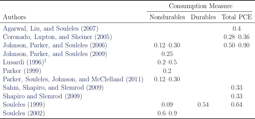
However, this is still at best only at the lower bound of typical empirical MPC
estimates which are typically between
-Dist model there are more households who possess less wealth,
are more impatient, and have higher MPCs (Figure 1 and dashed lines in
Figure 2).
However, this is still at best only at the lower bound of typical empirical MPC
estimates which are typically between  –
– or even higher (see Table 13 in
the Appendix E).
or even higher (see Table 13 in
the Appendix E).
Table 7: Average Marginal Propensity to Consume in Annual Terms
Thus far, we have been using total household net worth as our measure of
wealth. Implicitly, this assumes that all of the household’s debt and asset
positions are perfectly liquid and that, say, a household with home equity of
$50,000 and bank balances of $2,000 (and no other balance sheet items) will
behave in every respect similarly to a household with home equity of $10,000 and
bank balances of $42,000. This seems implausible. The home equity is
more illiquid (tapping it requires, at the very least, obtaining a home
equity line of credit, which requires an appraisal of the house and some
paperwork).
Otsuka (2003) formally analyzes the optimization problem of a consumer with
a FBS income process who can invest in an illiquid but higher-return asset
(think housing), or a liquid but lower-return asset (cash), and shows,
unsurprisingly, that the marginal propensity to consume out of shocks to liquid
assets is higher than the MPC out of shocks to illiquid assets. Her results would
presumably be even stronger if she had allowed that households hold so much of
their wealth in illiquid forms (housing, pension savings), for example, as a
mechanism to overcome self-control problems (see Laibson (1997) and many
others).
These considerations suggest that it may be more plausible, for purposes of
extracting a predictions about the MPC out of stimulus checks, to focus on
matching the distribution of liquid financial assets across households (that is,
assets which are of the same kind as represented by the stimulus check, once it
has been deposited into a bank account).
When we ask the model to estimate the time preference factors that allow it
to best match the distribution of liquid financial assets (instead of net
worth),
estimated parameter values are  and the average
MPC is
and the average
MPC is  (third column of the table), which lies in the upper part of the
range typically reported in the literature (see Table 13), and is considerably
higher than when we match the distribution of net worth. This reflects the fact
that matching the more skewed distribution of liquid financial assets than that of
net worth (Table 8) requires a wider distribution of the time preference factors,
which produces even more households with little wealth. The estimated
distribution of discount factors lies below that obtained by matching net worth
and is considerably more dispersed because of substantially lower median
and more unevenly distributed liquid financial wealth (compared to net
worth).
(third column of the table), which lies in the upper part of the
range typically reported in the literature (see Table 13), and is considerably
higher than when we match the distribution of net worth. This reflects the fact
that matching the more skewed distribution of liquid financial assets than that of
net worth (Table 8) requires a wider distribution of the time preference factors,
which produces even more households with little wealth. The estimated
distribution of discount factors lies below that obtained by matching net worth
and is considerably more dispersed because of substantially lower median
and more unevenly distributed liquid financial wealth (compared to net
worth).
Figure 3 shows the cumulative distribution functions of MPCs for the  -Dist
models estimated to match the empirical distribution of net worth and liquid
financial assets. The Figure illustrates the high values of implied MPCs obtained
for both models, especially the latter.
-Dist
models estimated to match the empirical distribution of net worth and liquid
financial assets. The Figure illustrates the high values of implied MPCs obtained
for both models, especially the latter.
MPCs are generally higher among low wealth/income households and
the unemployed in both our  -Point and
  -Dist models (rest of the
rows in Table 7). These results provide the basis for a common piece of
conventional wisdom about the effects of economic stimulus mentioned in our
introduction: If the purpose of the stimulus payments is to stimulate
consumption, it makes much more sense to target those payments to low-wealth
households than to distribute them uniformly to the population as a
whole.
-Dist models (rest of the
rows in Table 7). These results provide the basis for a common piece of
conventional wisdom about the effects of economic stimulus mentioned in our
introduction: If the purpose of the stimulus payments is to stimulate
consumption, it makes much more sense to target those payments to low-wealth
households than to distribute them uniformly to the population as a
whole.
4 A More Plausible and More Tractable ‘Friedman/Buffer Stock’ Aggregate
Process
The KS process for aggregate productivity shocks has little empirical foundation;
indeed, it appears to have been intended by the authors as an illustration of how
one might incorporate business cycles in principle, rather than a serious
candidate for an empirical description of actual aggregate dynamics. In this
section, we introduce an aggregate income process that is considerably more
tractable than the KS aggregate process and is also a much closer match to the
aggregate data. We regard the version of our model with this new income
process as the ‘preferred’ version for use as a starting point for future
research.
The aggregate production function is the same as equation (1), but following
Carroll, Slacalek, and Tokuoka (2008), the aggregate state (good or bad) no
longer exists in this model ( ). Aggregate productivity is instead captured
by
). Aggregate productivity is instead captured
by  . Specifically,
  ;
;  is aggregate permanent productivity, where
 ;
;  is the aggregate permanent shock; and
  is the
aggregate transitory shock (note that
is the
aggregate transitory shock (note that  is the capitalized version of the Greek
letter
is the capitalized version of the Greek
letter  used for the idiosyncratic permanent shock; similarly (though less
obviously),
used for the idiosyncratic permanent shock; similarly (though less
obviously),  is the capitalized
  ). Both
  and
and  are assumed to be log
normally distributed with mean one, and their log variances are from Carroll,
Slacalek, and Tokuoka (2008), who have estimated them using U.S. data
(Table 5).
are assumed to be log
normally distributed with mean one, and their log variances are from Carroll,
Slacalek, and Tokuoka (2008), who have estimated them using U.S. data
(Table 5).
Table 9: Aggregate Statistics in  -Dist Model under ‘Plausible’ Aggregate Process
The assumption that the structure of aggregate shocks resembles the structure
of idiosyncratic shocks is valuable not only because it matches the data better,
but also because it makes the model easier to solve. In particular, the elimination
of the ‘good’ and ‘bad’ aggregate states reduces the number of state variables to
two ( and
and  ) after normalizing the model by
  (as elaborated in
Carroll, Slacalek, and Tokuoka (2008)). As in Section 2, employment status is
not a state variable (in eliminating the aggregate states, we also shut down
unemployment persistence, which depends on the aggregate state in the
KS-JEDC or KS-Orig model). As before, the main thing the household
needs to know is the law of motion of
(as elaborated in
Carroll, Slacalek, and Tokuoka (2008)). As in Section 2, employment status is
not a state variable (in eliminating the aggregate states, we also shut down
unemployment persistence, which depends on the aggregate state in the
KS-JEDC or KS-Orig model). As before, the main thing the household
needs to know is the law of motion of  , which can be obtained by
following essentially the same method as described in the Appendix
C.
, which can be obtained by
following essentially the same method as described in the Appendix
C.
When matching the distribution of net worth, aggregate statistics produced by
the  -Dist model with our preferred (Friedman/Buffer Stock) aggregate process
are relatively similar to those under the KS aggregate process, despite the
difference in the aggregate process (first and third columns of Table 9). Given
that there is no aggregate state in the economy, we are using
-Dist model with our preferred (Friedman/Buffer Stock) aggregate process
are relatively similar to those under the KS aggregate process, despite the
difference in the aggregate process (first and third columns of Table 9). Given
that there is no aggregate state in the economy, we are using  and
and  estimated in Section 2 and assuming that the unemployment rate
  is fixed at
0.07 (same as in Section 2). Our preferred version of the
is fixed at
0.07 (same as in Section 2). Our preferred version of the  -Dist model
maintains positive
-Dist model
maintains positive  , and high correlation of consumption
growth with income growth or interest rates. We have obtained similar results by
matching the distribution of liquid financial assets (second column of the
table).
, and high correlation of consumption
growth with income growth or interest rates. We have obtained similar results by
matching the distribution of liquid financial assets (second column of the
table).
More importantly, the preferred version of the  -Dist model can
produce high MPCs. For example, in the net worth case, the average MPC
is
-Dist model can
produce high MPCs. For example, in the net worth case, the average MPC
is  , which is very close to the estimate under the KS aggregate
process (compare second and last but one columns of Table 7). In the
liquid financial assets case, the average MPC is higher at
, which is very close to the estimate under the KS aggregate
process (compare second and last but one columns of Table 7). In the
liquid financial assets case, the average MPC is higher at  (last
column).
(last
column).
5 Conclusion
This paper found that the performance of a KS-type model in replicating
wealth distribution can be improved significantly by introducing i) a
microfounded income process, ii) finite lifetimes, and iii) heterogeneity in time
preference factors. Moreover, such modifications improve macroeconomic
characteristics of the model by substantially boosting the MPC out of transitory
income.
A Derivation of Variance of Permanent Income
The evolution of the square of  is given by
where  if household
  dies.
dies.
Because ![2
Et [(1 - dt+1,i) ] = 1 - D](BSinKS332x.png) and
and ![2
Et [d t+1,i] = D](BSinKS333x.png) , we have
, we have
and
Finally, the steady state expected level of ![M [p2] ≡ lim M [p2]
t→ ∞ t](BSinKS336x.png) can be found
from
can be found
from
B Estimating Moffitt and Gottschalk Income Process
This appendix estimates the annual income process à la Moffitt and
Gottschalk (1995) using quarterly income draws generated by our income
process (Section 2) with parameter values from Table 1. Moffitt and
Gottschalk (1995) assume log permanent income  follows a
random walk and log transitory income
follows a
random walk and log transitory income  ) an ARMA process:
Like
Moffitt and Gottschalk (1995), we match the covariance matrix of the annual
income draws, and obtain estimate with the same signs as theirs obtained using
the PSID data; see Table 10, confirming that our calibration is qualitatively
consistent with Moffitt and Gottschalk’s.
Interestingly, even though our true quarterly transitory shock process is just
white noise, if we estimate the process on an annual basis we obtain
positive AR ( ) and negative MA (
 ) coefficients, reflecting time
aggregation. This suggests that the positive
) coefficients, reflecting time
aggregation. This suggests that the positive  and negative
  reported
in Moffitt and Gottschalk (1995) may be (at least) partly due to time
aggregation.
reported
in Moffitt and Gottschalk (1995) may be (at least) partly due to time
aggregation.
Table 10: Estimates of Moffitt and Gottschalk Annual Income Process
C Solution Method to Obtain Law of Motion
C.1 Solution Methods
Broadly speaking, the literature takes one of the following two approaches in
solving the KS problem in Section 3:
- Relying on simulation to obtain the law of motion of per capita capital
- (In principle) not relying on simulation to obtain the law of motion of
per capita capital
Table 11 lists some existing articles that solve the KS-JEDC model
according to this categorization. All articles in the table except Kim, Kim,
and Kollmann (2010) solve the exact KS-JEDC model using various
methods.
The advantage of the first approach is that simulation performed to obtain the
law of motion generates micro data, which can be used directly to investigate
issues such as wealth distribution. The disadvantage is that this approach
is generally subject to cross-sectional sampling variation, because this
approach typically performs simulation using a finite number of households.
Young (2010) and Den Haan (2010b)’s approaches can also be categorized in
the first approach but avoid cross-sectional sampling variation by running
nonstochastic simulation that approximates the density of wealth with a
histogram.
The advantages of the second approach are: i) there is no cross-sectional
sampling variation; ii) it is generally faster than the first approach.
Using the second approach, Algan, Allais, and Den Haan (2008)
and Reiter (2010) find a wealth distribution function of various
moments,
while Reiter (2010) calculates a matrix for the transition probabilities of
individual wealth (see Appendix ?? for details about his technique). Kim, Kim,
and Kollmann (2010) use a perturbation method that linearizes the system.
Although they are not able to solve the exact same KS-JEDC model and thus
modify the form of the utility function, they can solve a related problem very
quickly.
We use the first approach because it directly generates various micro data
(e.g., individual wealth and MPC), which can be used to examine wealth
distribution and the aggregate MPC. Details about our algorithm are in the next
subsection.
Table 11: Methods of Solving KS-JEDC Model
C.2 Our Algorithm
In solving the problem in section 3 we closely follow the stochastic simulation
method of Krusell and Smith (1998). Krusell and Smith find that per capita
capital today ( ) is sufficient to predict per capita capital tomorrow (
 ).
Our procedure is as follows:
).
Our procedure is as follows:
- Solve for the optimal individual decision rules given some ‘beliefs’
 that
determine the (expected) law of motion of per capita capital. The law of
motion is takes the log-linear form given by
that
determine the (expected) law of motion of per capita capital. The law of
motion is takes the log-linear form given by  :
:
if the aggregate state in period  is good (
 ), and
if the aggregate state is bad ( ).
).
- Simulate the economy populated by
 households (which experiments
determined is enough to suppress idiosyncratic noise) for
households (which experiments
determined is enough to suppress idiosyncratic noise) for  periods (following Maliar, Maliar, and Valli (2010)). When starting a
simulation,
periods (following Maliar, Maliar, and Valli (2010)). When starting a
simulation,  for all
  , the distribution of
  is generated
assuming
is generated
assuming  is equal to its steady state level (
 ) for all
  , and
, and
 (the aggregate state is good). (The steady state level of
 is
is  . With
  for all
  ,
,
 .) The newborn households start life with
  and
and
 .
.
- Estimate
 , which determines the law of motion of per capita capital,
using the last
, which determines the law of motion of per capita capital,
using the last  periods of data generated by the simulation (we
discard the first
periods of data generated by the simulation (we
discard the first  periods).
- Compute an improved vector for the next iteration by
 is used for the
  -Dist model. (Our experiments found that we
can reach the solution faster with
-Dist model. (Our experiments found that we
can reach the solution faster with  .)
.)
We repeat this process until  with a given degree of
precision.
with a given degree of
precision.
From the second iteration and thereafter, we use the terminal distribution of wealth
(and permanent component of income ( )) in the previous iteration as the initial
one. For the case of the
)) in the previous iteration as the initial
one. For the case of the  -Dist model, the number of households is multiplied
by 10 in the final two (or three) iterations to reduce cross-sectional simulation
error.
-Dist model, the number of households is multiplied
by 10 in the final two (or three) iterations to reduce cross-sectional simulation
error.
While we can eventually obtain some solution whatever the initial
 is, we use
  obtained using the representative agent model as the
starting point. This can significantly reduce the time needed to obtain the
solution.
obtained using the representative agent model as the
starting point. This can significantly reduce the time needed to obtain the
solution.
Parameter values to solve the model are from Table 1 (except for the
unemployment rate  ) and Table 5. The time preference factors are imposed
to be those estimated in Section 2.
) and Table 5. The time preference factors are imposed
to be those estimated in Section 2.
C.3 Tricks to Reduce Simulation Errors
In obtaining the aggregate law, we introduce the following tricks to reduce
simulation errors (or to speed up the solution given a degree of estimate
precision):
- Death: When death is concentrated among households at the very
top of the wealth distribution, per capita capital would be at a lower
than normal level. To alleviate simulation errors from this source, each
period we: i) sort households by wealth level, ii) construct groups,
the size of which is the inverse of the death probability (under our
parameter choice, the size of each group is 200 and the first group
contains households from the wealthiest to the 200th), and iii) pick one
household that dies within each group.
- Permanent income shocks: In our methodology, permanent shocks
to income are approximated by
 discrete points. Similarly to the
death element, after sorting we set up groups each of size
discrete points. Similarly to the
death element, after sorting we set up groups each of size  . We
randomize shocks within each group subject to the constraint that
each shock point is experienced by one of the group members every
period, making the group mean of the shocks equal to the theoretical
mean.
. We
randomize shocks within each group subject to the constraint that
each shock point is experienced by one of the group members every
period, making the group mean of the shocks equal to the theoretical
mean.
C.4 Estimated Laws of Motion
The estimated laws of motions for  -Point,
  -Dist and KS-JEDC models are
given in Table 12. The fit measured with
-Dist and KS-JEDC models are
given in Table 12. The fit measured with  in all specifications exceeds
0.9999.
in all specifications exceeds
0.9999.
Table 12: Estimated Laws of Motion
Notes: The coefficients for the KS-JEDC model are very close to those estimated in Maliar, Maliar, and
Valli (2010).
D Experiment to Understand Sticky Consumption Growth in KS-JEDC
Model
Although  reported in subsection 3.1 may not be high
enough relative to that observed in the U.S. data, it is still not clear why
simulations produce such a high value.
reported in subsection 3.1 may not be high
enough relative to that observed in the U.S. data, it is still not clear why
simulations produce such a high value.
Previous studies on KS type models have not investigated this issue. Using
the KS-JEDC model, we performed an experiment to understand the
phenomenon better. In this experiment we assume that the aggregate
state switches from good to bad (or from bad to good) every eight
quarters.
Figure 4 plots  24 quarters of simulated observations (the state is
bad for the first eight quarters, good for the next eight quarters, and bad for the
final eight quarters). The figure shows that
24 quarters of simulated observations (the state is
bad for the first eight quarters, good for the next eight quarters, and bad for the
final eight quarters). The figure shows that  is very persistent (it is
negative in the bad state and positive in the good state), resulting in a relatively
high
is very persistent (it is
negative in the bad state and positive in the good state), resulting in a relatively
high  .
.
It is easy to understand that  is higher when the state is good (and
vice versa) given the following facts:
is higher when the state is good (and
vice versa) given the following facts:
- A first order approximation of the Euler equation yields:
 | (20) |
where  ,
,  ,
,  is the coefficient of
relative risk aversion,
is the coefficient of
relative risk aversion,  is the interest rate,
  is the time
preference factor, and
is the time
preference factor, and  is the depreciation rate. Indeed, when
we conduct an IV regression of equation (20) using
is the depreciation rate. Indeed, when
we conduct an IV regression of equation (20) using  as the
instrument,
which effectively means estimating
as the
instrument,
which effectively means estimating ![Δ log CCCt = b0 + b1 Et - 1 [rt] + εt](BSinKS413x.png) , the
estimate of
, the
estimate of  is
is  (with a standard deviation of
  ) and
relatively close to the actual value of
) and
relatively close to the actual value of  (
( ). This suggests
that using the predictable component of interest rates (
). This suggests
that using the predictable component of interest rates (![E [r ]
t- 1 t](BSinKS419x.png) ),
we can obtain a reasonable estimate of intertemporal elasticity of
substitution.
),
we can obtain a reasonable estimate of intertemporal elasticity of
substitution.
- When the state is good,
 (from (19)) is higher
because
(from (19)) is higher
because  (aggregate productivity) is higher, as can be seen in Figure 5,
which plots the dynamics of
(aggregate productivity) is higher, as can be seen in Figure 5,
which plots the dynamics of  for the 24 quarters.
While in typical simulation one state does not generally last for exactly eight
quarters, we observe sticky aggregate consumption growth (and a relatively high
 ) because the same mechanisms are at work as in the
experiment above.
) because the same mechanisms are at work as in the
experiment above.
In sum, a relatively high  in the KS-JEDC model can
be interpreted as a consequence of the persistent behavior of the interest rate
in the KS-JEDC model can
be interpreted as a consequence of the persistent behavior of the interest rate
 . Indeed, denoting
 ![εt = Δ log CCCt - b0 - b1 Et - 1[rt]](BSinKS426x.png) the residual after
controlling for the predictable component of consumption growth related
to interest rates, we find that
the residual after
controlling for the predictable component of consumption growth related
to interest rates, we find that  0.02 is much lower than
 .
.
E Empirical Estimates of MPCs
Table 13 summarizes the estimates of MPCs obtained using household-level data
on various recent fiscal stimulus measures in the U.S.
Table 13: Estimates of MPCs
Notes:  : elasticity.
References
AGARWAL, SUMIT, CHUNLIN LIU, AND NICHOLAS S. SOULELES
(2007): “The Response of Consumer Spending and Debt to Tax Rebates
– Evidence from Consumer Credit Data,” Journal of Political Economy,
115(6), 986–1019.
ALGAN, YANN, OLIVER ALLAIS, AND WOUTER J. DEN HAAN
(2008): “Solving Heterogeneous-agent Models with Parameterized
Cross-sectional Distributions,” Journal of Economic Dynamics and
Control, 32(3), 875–908.
BEWLEY, TRUMAN (1977): “The Permanent Income Hypothesis: A
Theoretical Formulation,” Journal of Economic Theory, 16, 252–292.
BLANCHARD, OLIVIER J. (1985): “Debt, Deficits, and Finite
Horizons,” Journal of Political Economy, 93(2), 223–247.
BLUNDELL, RICHARD, LUIGI PISTAFERRI, AND IAN PRESTON
(2008): “Consumption Inequality and Partial Insurance,” Manuscript.
BRAUN, RICHARD ANTON, HUIYU LI, AND JOHN STACHURSKI
(2009): “Computing Densities and Expectations in Stochastic Recursive
Economies: Generalized Look-Ahead Techniques,” Manuscript.
CAGETTI, MARCO (2003): “Wealth Accumulation Over the Life Cycle
and Precautionary Savings,” Journal of Business and Economic Statistics,
21(3), 339–353.
CAMPBELL, JOHN Y., AND N. GREGORY MANKIW
(1989): “Consumption, Income, and Interest Rates: Reinterpreting the
Time-Series Evidence,” in NBER Macroeconomics Annual, 1989, ed.
by Olivier J. Blanchard, and Stanley Fischer, pp. 185–216. MIT Press,
Cambridge, MA, http://ideas.repec.org/p/nbr/nberwo/2924.html.
__________ (1991): “The Response of Consumption to Income: A
Cross-Country Investigation,” European Economic Review, 35, 723–67.
CARROLL, CHRISTOPHER D. (1992): “The Buffer-Stock Theory of
Saving: Some Macroeconomic Evidence,” Brookings Papers on Economic
Activity, 1992(2), 61–156,
http://www.econ2.jhu.edu/people/ccarroll/BufferStockBPEA.pdf.
__________ (2000a): “Requiem for the Representative Consumer?
Aggregate Implications of Microeconomic Consumption Behavior,”
American Economic Review, 90(2), 110–115.
__________ (2000b): “Why Do the Rich Save So Much?,” in Does Atlas
Shrug? The Economic Consequences of Taxing the Rich, ed. by Joel B.
Slemrod. Harvard University Press,
http://www.econ2.jhu.edu/people/ccarroll/Why.pdf.
__________ (2011): “Theoretical Foundations of Buffer Stock Saving,”
Manuscript, Department of Economics, Johns Hopkins University,
http://www.econ2.jhu.edu/people/ccarroll/papers/BufferStockTheory.
CARROLL, CHRISTOPHER D., AND ANDREW A. SAMWICK (1997):
“The Nature of Precautionary Wealth,” Journal of Monetary Economics,
40(1), 41–71.
CARROLL, CHRISTOPHER D., JIRI SLACALEK,
AND KIICHI TOKUOKA (2008): “Sticky Expectations and Consumption
Dynamics,” Manuscript.
CARROLL, CHRISTOPHER D., MARTIN SOMMER, AND
JIRI SLACALEK (2011): “International Evidence on Sticky Consumption
Growth,” Review of Economics and Statistics, 93(4), 1135–1145,
http://www.econ2.jhu.edu/people/ccarroll/papers/cssIntlStickyC/.
CASTANEDA, ANA, JAVIER DIAZ-GIMENEZ, AND JOSE-VICTOR
RIOS-RULL (2003): “Accounting for the U.S. Earnings and Wealth
Inequality,” Journal of Political Economy, 111(4), 818–857.
CORONADO, JULIA LYNN, JOSEPH P. LUPTON, AND LOUISE M.
SHEINER (2005): “The Household Spending Response to the 2003 Tax
Cut: Evidence from Survey Data,” FEDS discussion paper 32, Federal
Reserve Board.
DEATON, ANGUS S. (1991): “Saving and Liquidity Constraints,”
Econometrica, 59, 1221–1248.
DEN HAAN, WOUTER J. (2010a): “Assessing the Accuracy of the
Aggregate Law of Motion in Models with Heterogeneous Agents,” Jouranl
of Economic Dynamics and Control, 34(1), 79–99.
__________ (2010b): “Comparison of Solutions to the Incomplete Markets
Model with Aggregate Uncertainty,” Journal of Economic Dynamics and
Control, 34(1), 4–27.
DEN HAAN, WOUTER J., AND PONTUS RENDAHL (2010): “Solving
the Incomplete Markets Model with Aggregate Uncertainty Using Explicit
Aggregation,” Journal of Economic Dynamics and Control, 34(1), 69–78.
DIAMOND, PETER A. (1965): “National Debt in a Neoclassical Growth
Model,” American Economic Review, 55, 1126–1150.
FRIEDMAN, MILTON A. (1957): A Theory of the Consumption
Function. Princeton University Press.
FUHRER, JEFFREY C. (2000): “Habit Formation in Consumption
and its Implications for Monetary Policy Models,” American Economic
Review, 90(3), 367–390, http://www.jstor.org/stable/117334.
GORMAN, WILLIAM M. (1953): “Community Preference Fields,”
Econometrica, 21(1), 63–80.
GUVENEN, FATIH (2007): “Learning Your Earning: Are Labor Income
Shocks Really Very Persistent?,” American Economic Review, 97(3),
687–712.
__________ (2009): “An Empirical Investigation of Labor Income
Processes,” Review of Economic Dynamics, 12.
HALL, ROBERT E. (1978): “Stochastic Implications of
the Life-Cycle/Permanent Income Hypothesis: Theory and
Evidence,” Journal of Political Economy, 96, 971–87, Available at
http://www.stanford.edu/~rehall/Stochastic-JPE-Dec-1978.pdf.
__________ (1988): “Intertemporal Substitution in Consumption,”
Journal of Political Economy, XCVI, 339–357, Available at
http://www.stanford.edu/~rehall/Intertemporal-JPE-April-1988.pdf.
HRYSHKO, DMYTRO (2010): “RIP to HIP: The Data Reject
Heterogeneous Labor Income Profiles,” Manuscript, University of Alberta.
HUBBARD, R. GLENN, JONATHAN S. SKINNER, AND STEPHEN P.
ZELDES (1994): “The Importance of Precautionary Motives for Explaining
Individual and Aggregate Saving,” in The Carnegie-Rochester Conference
Series on Public Policy, ed. by Allan H. Meltzer, and Charles I. Plosser,
vol. 40, pp. 59–126.
JENSEN, SHANE T., AND STEPHEN H. SHORE (2008): “Changes in
the Distribution of Income Volatility,” Manuscript.
JOHNSON, DAVID S., JONATHAN A. PARKER, AND NICHOLAS S.
SOULELES (2006): “Household Expenditure and the Income Tax Rebates
of 2001,” American Economic Review, 96(5), 1589–1610.
__________ (2009): “The Response of Consumer Spending to Rebates
During an Expansion: Evidence from the 2003 Child Tax Credit,” working
paper, The Wharton School.
KAPLAN, GREG, AND GIOVANNI L. VIOLANTE (2011): “A Model of
the Consumption Response to Fiscal Stimulus Payments,” NBER Working
Paper Number W17338.
KENNICKELL, ARTHUR B. (1995): “Saving and Permanent Income:
Evidence from the 1992 SCF,” Board of Governors of the Federal Reserve
System.
KIM, JINILL, SUNGHYUN HENRY KIM, AND ROBERT KOLLMANN
(2010): “Solving the Incomplete Market Model with Aggregate
Uncertainty Using a Perturbation Method,” Journal of Economic
Dynamics and Control, 34(1), 50–58.
KIRMAN, ALAN P. (1992): “Whom or What Does the Representative
Individual Represent?,” The Journal of Economic Perspectives, 6(2),
117–136.
KRUSELL, PER, AND ANTHONY A. SMITH (1998): “Income and
Wealth Heterogeneity in the Macroeconomy,” Journal of Political
Economy, 106(5), 867–896.
LAIBSON, DAVID (1997): “Golden Eggs and Hyperbolic Discounting,”
Quarterly Journal of Economics, CXII(2), 443–477.
LOW, HAMISH, COSTAS MEGHIR, AND LUIGI PISTAFERRI (2005):
“Wage Risk and Employment Over the Life Cycle,” Manuscript, Stanford
University.
LUCAS, ROBERT E. (1976): “Econometric Policy Evaluation: A
Critique,” in The Phillips Curve and Labour Markets, ed. by Karl
Brunner, and Allan H. Meltzer, vol. 1, pp. 19–46. Journal of Monetary
Economics (Supplement).
LUSARDI, ANNAMARIA (1996): “Permanent Income, Current Income,
and Consumption: Evidence from Two Panel Data Sets,” Journal of
Business and Economic Statistics, 14(1), 81–90.
MACURDY, THOMAS (1982): “The Use of Time Series Processes to
Model the Error Structure of Earnings in a Longitudinal Data Analysis,”
Journal of Econometrics, 18(1), 83–114.
MALIAR, LILIA, SERGUEI MALIAR, AND FERNANDO VALLI (2008):
“Comparing Numerical Solutions of Models with Heterogeneous Agents
(Models B): a Grid-based Euler Equation Algorithm,” Manuscript.
__________ (2010): “Solving the Incomplete Markets Model with Aggregate
Uncertainty Using the Krusell Smith Algorithm,” Journal of Economic
Dynamics and Control, 34(1), 42–49.
MEGHIR, COSTAS, AND LUIGI PISTAFERRI (2004): “Income Variance
Dynamics and Heterogeneity,” Journal of Business and Economic
Statistics, 72(1), 1–32.
MODIGLIANI, FRANCO, AND RICHARD BRUMBERG (1954): “Utility
Analysis and the Consumption Function: An Interpretation of
Cross-Section Data,” in Post-Keynesian Economics, ed. by Kenneth K.
Kurihara, pp. 388–436. Rutgers University Press, New Brunswick, N.J.
MOFFITT, ROBERT A., AND PETER GOTTSCHALK (1995): “Trends in
the Covariance Structure of Earnings in the U.S.: 1969-1987,” Manuscript.
NIELSEN, HELENA SKYT, AND ANNETTE VISSING-JORGENSEN
(2006): “The Impact of Labor Income Risk on Educational Choices:
Estimates and Implied Risk Aversion,” Manuscript.
OTSUKA, MISUZU (2003): “Household Portfolio Choice with Illiquid
Assets,” manuscript, Johns Hopkins University.
PARKER, JONATHAN A. (1999): “The Reaction of Household
Consumption to Predictable Changes in Social Security Taxes,” American
Economic Review, 89(4), 959–973.
PARKER, JONATHAN A., NICHOLAS S. SOULELES, DAVID S.
JOHNSON, AND ROBERT MCCLELLAND (2011): “Consumer Spending
and the Economic Stimulus Payments of 2008,” NBER Working Paper
Number W16684.
REITER, MICHAEL (2010): “Solving the Incomplete Markets Model with
Aggregate Uncertainty by Backward Induction,” Journal of Economic
Dynamics and Control, 34(1), 28–35.
SABELHAUS, JOHN, AND JAE SONG (2010): “The Great Moderation in
Micro Labor Earnings,” Journal of Monetary Economics, 57(4), 391–403,
http://ideas.repec.org/a/eee/moneco/v57y2010i4p391-403.html.
SAHM, CLAUDIA R., MATTHEW D. SHAPIRO, AND JOEL B.
SLEMROD (2009): “Household Response to the 2008 Tax Rebate: Survey
Evidence and Aggregate Implications,” NBER Working Paper Number
W15421.
SAMUELSON, PAUL A. (1958): “An exact consumption loan model of
interest with or without the social contrivance of money,” Journal of
Political Economy, 66, 467–482.
SHAPIRO, MATTHEW W., AND JOEL B. SLEMROD (2009): “Did the
2008 Tax Rebates Stimulate Spending?,” American Economic Review,
99(2), 374–379.
SOLOW, ROBERT M. (2003): “Dumb and Dumber in Macroeconomics,”
Manuscript, MIT.
SOULELES, NICHOLAS S. (1999): “The Response of Household
Consumption to Income Tax Refunds,” American Economic Review,
89(4), 947–958.
__________ (2002): “Consumer Response to the Reagan Tax Cuts,” Journal
of Public Economics, 85, 99–120.
STORESLETTEN, KJETIL, CHRIS I. TELMER, AND AMIR YARON
(2004a): “Consumption and Risk Sharing Over the Life Cycle,” Journal
of Monetary Economics, 51(3), 609–633.
__________ (2004b): “Cyclical Dynamics in Idiosyncratic Labor-Market
Risk,” Journal of Political Economy, 112(3), 695–717.
SZEIDL, ADAM (2006): “Invariant Distribution in Buffer-Stock Saving
and Stochastic Growth Models,” Manuscript, University of California at
Berkeley.
TOPEL, ROBERT H. (1990): “Specific Capital, Mobility and Wages:
Wages Rise with Job Seniority,” NBER Working Paper Number W3294.
TOPEL, ROBERT H., AND MICHAEL P. WARD (1992): “Job Mobility
and the Careers of Young Men,” Quarterly Journal of Economics, 107(2),
439–479.
YOUNG, ERIC R. (2010): “Solving the Incomplete Markets Model
with Aggregate Uncertainty Using the Krusell-Smith Algorithm and
Non-Stochastic Simulations,” Journal of Economic Dynamics and
Control, 34(1), 36–41.
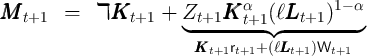
![[ 1- ρ ]
V (Mt, Zt ) = max u(Ct ) + β Et Γt+1 V (Mt+1, Zt+1 ) (2)
Ct
s.t.
At = Mt - Ct (3)
Kt+1 = At ∕Γ t+1 (4)
Mt+1 = ℸKt+1 + K α , (5)
t+1](BSinKS26x.png)
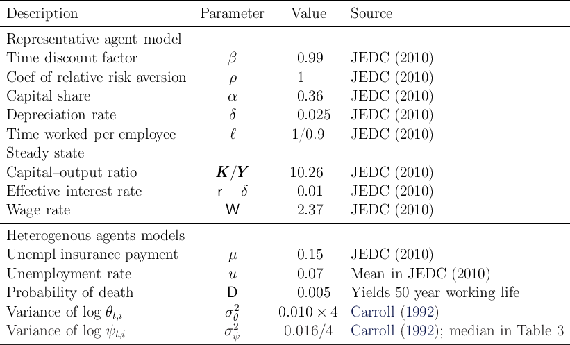

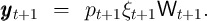
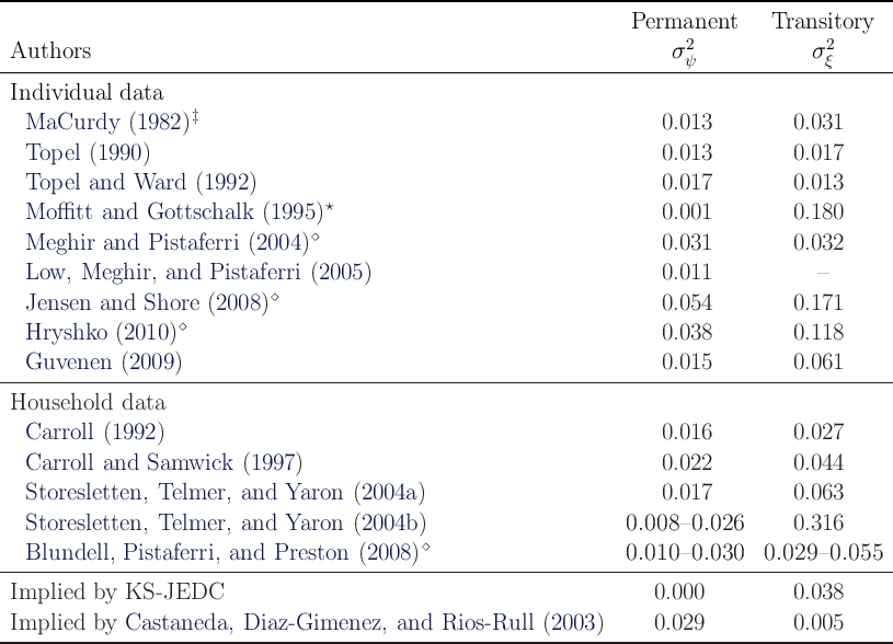
![D
M [p2] = -------------- (7)
1 - //D E [ψ2 ]](BSinKS88x.png)
![2 2
σ p = M [p ] - 1.](BSinKS90x.png)
![------------------------------------------------------
Dataset var (p) E [ψ2 ] σ2
-------------------------------------------------ψ----
SCF1992 2.5 1.015 0.015
SCF1995 7.5 1.018 0.018
SCF1998 3.1 1.015 0.015
SCF2001 3.6 1.016 0.016
SCF2004 5.2 1.017 0.017
------------------------------------------------------
KS -Orig or KS -JEDC 0 1 0
------------------------------------------------------](BSinKS99x.png)
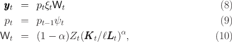
![[ 1- ρ ]
v(mt ) = max u (ct) + β//D Et ψt+1 v(mt+1 ) (13)
ct
s.t.
at = mt - ct
at ≥ 0
k = a ∕(//D ψ ) (14)
t+1 t t+1
mt+1 = (ℸ + r)kt+1 + ξt+1 (15)](BSinKS130x.png)
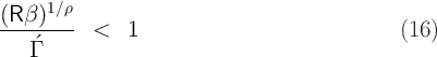
![( - ρ )- 1∕ρ
´Γ = E [ψ ] Γ .](BSinKS163x.png)


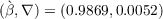


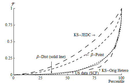
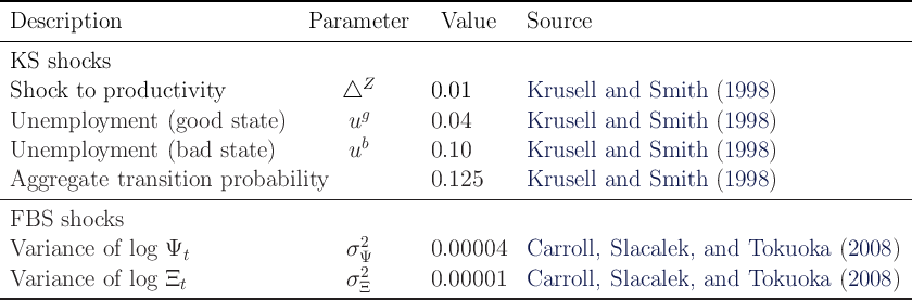
![[ 1- ρ ]
v(mt, ιt;KKKt, Zt ) = maxc u(ct) + β/D/ Et (Γ t+1 ψt+1 ) v (mt+1, ιt;KKKt+1, Zt+1 )
t
s.t.
a = m - c
t t t
at ≥ 0
kt+1 = at∕ (//D Γ t+1 ψt+1 )
mt+1 = (ℸ + rt+1 )kt+1 + yt+1
r = αZ (KKK ∕ℓLLL )α- 1, (19)
t+1 t+1 t+1 t+1](BSinKS234x.png)
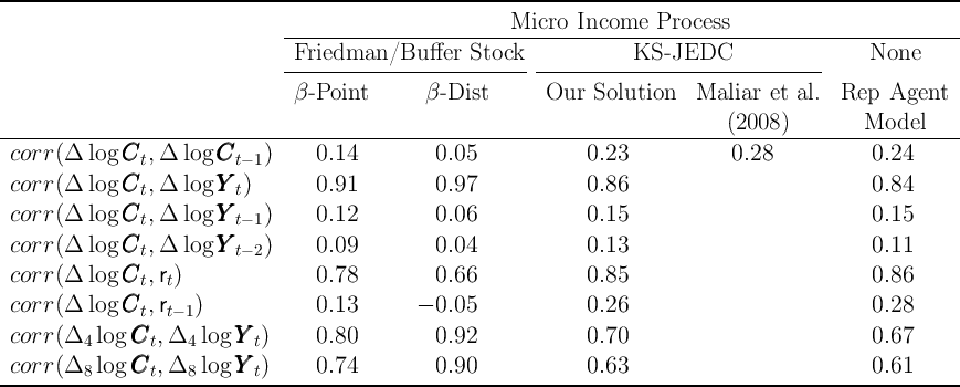
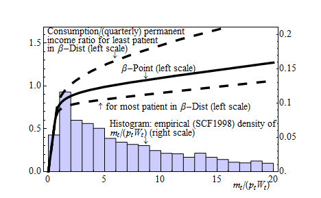
 -Point and
  -Dist Models
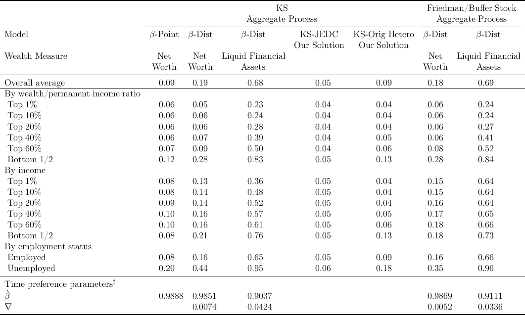


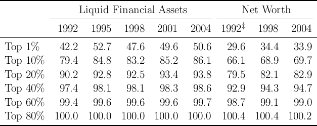

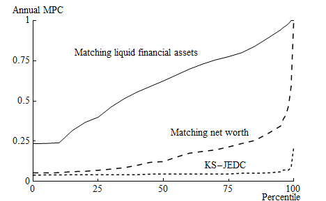
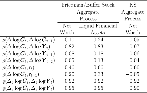
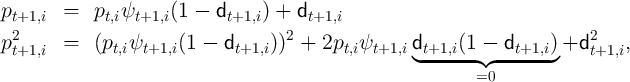
![Et[p2t+1,i] = Et [(pt,iψt+1,i(1 - dt+1,i))2] + D
2 2
= p t,i//D E [ψ ] + D,](BSinKS334x.png)
![[ 2 ] 2 2
M p t+1 = M [p t]/D/ E [ψ ] + D.](BSinKS335x.png)
![M [p2] = D + /D E [ψ2 ]M [p2]
/
2 ------D-------
M [p ] = / 2 .
1 - /D E [ψ ]](BSinKS337x.png)
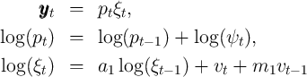
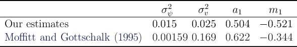
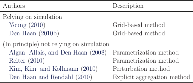

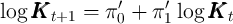
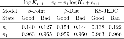
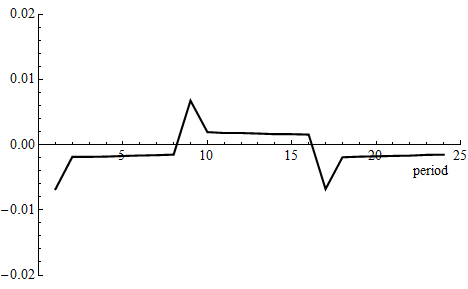
 in KS-JEDC Model
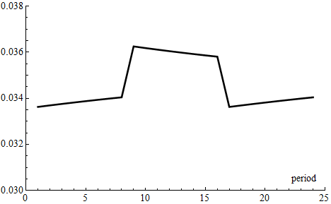
 in KS-JEDC Model