International Evidence On
Sticky Consumption Growth
July 1, 2010
| Christopher D. Carroll1 |
| . |
_____________________________________________________________________________________
Abstract
This paper estimates the degree of ‘stickiness’ in aggregate consumption
growth (sometimes interpreted as reflecting consumption habits) for thirteen
advanced economies. We find that, after controlling for measurement
error, consumption growth has a high degree of autocorrelation, with
a stickiness parameter of about 0.7 on average across countries. The
sticky-consumption-growth model outperforms the random walk model of
Hall (1978), and typically fits the data better than the popular Campbell and
Mankiw (1989) model, though in a few countries the sticky-consumption-growth
and Campbell–Mankiw models work about equally well.
-
Keywords
-
Consumption, Sticky Expectations, Habits
-
JEL codes
-
E21, F41
| | | (Contains data and estimation software producing paper’s results) |
1Carroll: Department of Economics, Johns Hopkins University, Baltimore, MD, http://www.econ2.jhu.edu/people/ccarroll/,
ccarroll@jhu.edu, Phone: (410) 516 7602 2Slacalek: European Central Bank, Frankfurt am Main, Germany,
http://www.slacalek.com/, jiri.slacalek@ecb.europa.eu, Phone: +49 69 1344 5047 3Sommer: International
Monetary Fund, Washington, DC, http://martinsommeronline.googlepages.com/, msommer@imf.org, Phone: (202) 623
9998
1 Introduction
A large literature ranging across macroeconomics, finance, and international economics
has argued that ‘habit formation’ can explain many empirical facts related to consumption
dynamics.
The core empirical pattern driving all these findings appears to be that
aggregate consumption growth is too ‘sticky’ to be explained with standard
models. Other explanations for the persistence of aggregate spending growth, or
‘excess smoothness’ (in Campbell and Deaton (1989)’s terminology), include
consumers’ inattentiveness to macroeconomic news (Sims (2003); Reis (2006);
Carroll and Slacalek (2007)), or their inability to distinguish micro- from
macro-economic shocks (Pischke (1995)). Further explanations could
undoubtedly be imagined.
But a full consensus has not emerged on whether empirical data are
irreconcilable with Hall (1978)’s benchmark random walk model of consumption.
Hall’s model implies that consumption growth is unpredictable (excess
smoothness is zero). However, standard extensions of the Hall model can
generate some degree of stickiness in consumption growth. For example, excess
smoothness might merely reflect the fact that spending decisions are made
more frequently than consumption data are measured (Working (1960);
this viewpoint has recently been advocated in papers by Ludvigson and
Lettau (2001); Lettau and Ludvigson (2004)). Also, in the presence of
uncertainty, the precautionary motive slows down consumers’ response to shocks,
which could also explain part (though not all) of the excess smoothness
(Ludvigson and Michaelides (2001)). Another possibility, not often mentioned
but nevertheless worth serious consideration, is that the smoothness of measured
spending reflects data construction methods (e.g. for components of spending for
which quarterly observations are imputed using annual data sources). Finally,
many of the papers in the habit formation literature have not carefully
examined the possibility that their results might reflect the presence of
some ‘rule-of-thumb’ consumers, who simply set consumption equal to
income in each period, as proposed in influential papers by Campbell and
Mankiw (1989, 1991).
Motivated by this debate and by the fact that much of the empirical evidence
on excess smoothness has come from a single country (the U.S.), this paper
provides systematic estimates of three simple canonical models of consumption
dynamics using data for all advanced economies for which we were able to
construct appropriate datasets (thirteen countries in all). We compare the
random walk model of Hall (1978) with two alternatives: the Campbell and
Mankiw (1989) model, and a model that permits (but does not require) excess
smoothness. We remain deliberately agnostic (in this paper) about whether such
smoothness reflects habits, inattention, or other factors; our aim is simply to
document the key stylized facts that should be matched by any model of
aggregate consumption dynamics.
Using both instrumental variables (IV) (section 3.1) and Kalman filter
structural (section 3.2) estimation methods, we find strong evidence of excess
smoothness (‘stickiness’) in consumption growth in every country in our
sample.
Although there is some variation across countries in the estimated degree of
stickiness, in every country we can reject the hypothesis that the stickiness
coefficient is zero (the random walk theory), while in no country can we reject
the hypothesis that it is 0.7 in quarterly data. Furthermore, wherever
there is a clear distinction between the two non-random-walk models,
the sticky consumption growth model outperforms the rule-of-thumb
model, usually by a decisive statistical margin. (In a few cases, the two
non-random-walk models are not statistically distinguishable from each
other.)
The large size of our estimated stickiness parameter may come as a surprise to
some readers, because the serial correlation coefficient for spending growth in the
raw data is much lower than 0.7 (for instance, in U.S. data the OLS estimate of
the AR(1) coefficient for nondurables and services consumption growth is about
0.35). The discrepancy reflects our use of econometric methods that are robust to
the presence of measurement error. Consistent with Sommer (2007)’s findings for
the United States, our estimates suggest that in most countries at least half of
the quarterly variation in consumption growth can be interpreted either as
measurement error or as truly transitory spending disturbances unrelated to the
theoretical consumption model (caused, for example, by unseasonal weather,
which can have a nontrivial effect at the quarterly frequency in most
countries).
The remainder of the paper is organized as follows. Section 2 outlines two
theoretical frameworks that generate sticky consumption growth and provide the
conceptual framework for our estimation strategy. Section 3 presents the main
empirical results and Section 4 concludes.
2 Two Theories of Stickiness
This section sketches the two most popular theoretical frameworks—habit
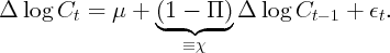
formation and sticky expectations—that can generate serial correlation in
aggregate consumption growth. In the habit formation model, the serial
correlation coefficient  reflects the strength of habits (if
  , the model
collapses to the Hall random walk model); in the sticky information model,
, the model
collapses to the Hall random walk model); in the sticky information model,
 is the fraction of aggregate expenditure by households that have
not fully updated their information set about the latest macroeconomic
developments (and again,
is the fraction of aggregate expenditure by households that have
not fully updated their information set about the latest macroeconomic
developments (and again,  corresponds to the Hall model).
Because the implications of the two frameworks are indistinguishable
in aggregate data, our empirical evidence is consistent with either
model.
corresponds to the Hall model).
Because the implications of the two frameworks are indistinguishable
in aggregate data, our empirical evidence is consistent with either
model.
2.1 Habit Formation
Muellbauer (1988) proposed a simple model of habit persistence, in which the
representative consumer maximizes time-nonseparable utility
 | (1) |
subject to the usual transversality condition and the dynamic budget
constraint:
 | (2) |
where  is the discount factor,
  is the consumption level,
  is market
resources (net worth plus current income),
is market
resources (net worth plus current income),  is the constant interest factor,
and
is the constant interest factor,
and  is noncapital income.
  in (1) represents the ‘habit stock,’ i.e., the
reference level of consumption to which the consumer compares the current
consumption level. The parameter
in (1) represents the ‘habit stock,’ i.e., the
reference level of consumption to which the consumer compares the current
consumption level. The parameter  captures the strength of habits. After
rewriting the utility function as
captures the strength of habits. After
rewriting the utility function as  , one
can see that, for
, one
can see that, for  , the consumer derives utility from both the level
and the change in consumption.
, the consumer derives utility from both the level
and the change in consumption.
Dynan (2000) shows that for a habit-forming consumer with Constant
Relative Risk Aversion (CRRA) outer utility 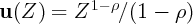 and
and
 , a first order approximation to the Euler equation leads to
consumption dynamics that satisfy:
, a first order approximation to the Euler equation leads to
consumption dynamics that satisfy:
 | (3) |
where  mainly reflects innovations to lifetime
resources.
Hence, in contrast to the standard intertemporally separable utility specification,
some of period
mainly reflects innovations to lifetime
resources.
Hence, in contrast to the standard intertemporally separable utility specification,
some of period  ’s consumption growth is predictable at time
  , and the
strength of habits
, and the
strength of habits  can be measured directly by estimating an AR(1)
regression like (3) on aggregate consumption data.
can be measured directly by estimating an AR(1)
regression like (3) on aggregate consumption data.
2.2 Sticky Expectations
Carroll and Slacalek (2007) present an alternative model that also generates
sticky aggregate consumption growth, but without departing from the
conventional intertemporally separable utility specification. The key assumption
is that consumers are mildly inattentive to macro developments—for
example, some households do not immediately notice shocks to aggregate
macroeconomic indicators such as productivity growth or the unemployment
rate.
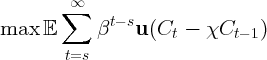
Assume that consumers maximize the discounted sum of time separable utility
 subject to the budget constraint (2). In a Hall (1978) model
with quadratic utility, in which households use all available information, the
optimal consumption level follows a random walk:
subject to the budget constraint (2). In a Hall (1978) model
with quadratic utility, in which households use all available information, the
optimal consumption level follows a random walk:  . Numerical
simulations in Carroll and Slacalek (2007) show that when quadratic utility is
replaced with CRRA utility and the model is solved with realistic calibrations of
idiosyncratic and aggregate uncertainty, the log of aggregate consumption is close
to a random walk with drift (the drift reflects the precautionary motive and the
attendant nonlinearities):
. Numerical
simulations in Carroll and Slacalek (2007) show that when quadratic utility is
replaced with CRRA utility and the model is solved with realistic calibrations of
idiosyncratic and aggregate uncertainty, the log of aggregate consumption is close
to a random walk with drift (the drift reflects the precautionary motive and the
attendant nonlinearities): 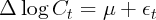 .
.
Suppose now that the economy consists of a continuum of inattentive but
otherwise-standard CRRA-utility consumers, each of whom updates the
information about his permanent income with probability  in each period. For
each consumer, this probability is assumed to be independent of the date when
he last updated his information set (and independent of his income, wealth,
or other characteristics). This assumption resembles firm behavior in
Calvo (1983)’s model of price setting, which is commonly used in the monetary
economics literature. Carroll and Slacalek (2007) show that the change in
the log of aggregate consumption,
in each period. For
each consumer, this probability is assumed to be independent of the date when
he last updated his information set (and independent of his income, wealth,
or other characteristics). This assumption resembles firm behavior in
Calvo (1983)’s model of price setting, which is commonly used in the monetary
economics literature. Carroll and Slacalek (2007) show that the change in
the log of aggregate consumption,  , approximately follows an
AR(1) process, whose autocorrelation coefficient approximates the share
of consumers (
, approximately follows an
AR(1) process, whose autocorrelation coefficient approximates the share
of consumers ( ) who do not have up-to-date information about
macroeconomic developments. That is, consumption growth is well approximated
by:
) who do not have up-to-date information about
macroeconomic developments. That is, consumption growth is well approximated
by:
 | (4) |
In addition, in the spirit of Akerlof and Yellen (1985) and Cochrane (1991), Carroll
and Slacalek (2007) show that the utility loss from the infrequent updating of
expectations is very small under standard calibrations of the model with  per
quarter.
per
quarter.
3 Empirical Results
This section tests the model of sticky consumption growth (3) and (4)
against the alternatives of rule-of-thumb behavior and the random
walk hypothesis. The organizing framework for our empirical analysis
is a specification for consumption growth from the excess sensitivity
literature,
which has been expanded here to include a term capturing stickiness of
consumption growth:
![Δ log C = ς + χ E [Δ log C ] + η E [Δ log Y ] + α E [a ] + ϵ ,
t t- 2 t- 1 t- 2 t t- 2 t- 1 t](cssIntlStickyC31x.png) | (5) |
where  is household income and
  denotes the ratio of household (net)
assets to permanent income. The first two right-hand side regressors correspond
to two of the tested theories of consumption behavior: inattentiveness or habit
formation (
denotes the ratio of household (net)
assets to permanent income. The first two right-hand side regressors correspond
to two of the tested theories of consumption behavior: inattentiveness or habit
formation ( ) and rule-of-thumb consumers (
 ). Under the
third tested theory—the random walk hypothesis—the coefficients
). Under the
third tested theory—the random walk hypothesis—the coefficients  and
and  should both be zero. The third term in the equation above (
 ) is included
as a control—any of the three theories allow for some direct effect of
asset holdings on consumption growth, either due to effects related to
uncertainty (which induces a precautionary saving motive) or due to time
variation in interest rates (which we assume is captured by time variation in
) is included
as a control—any of the three theories allow for some direct effect of
asset holdings on consumption growth, either due to effects related to
uncertainty (which induces a precautionary saving motive) or due to time
variation in interest rates (which we assume is captured by time variation in
 ).
).
There are at least three reasons to expect the OLS estimates of coefficients in
(5) to be biased and inconsistent. First, as argued by Wilcox (1992) and
Sommer (2007), quarterly consumption data may be contaminated with
substantial measurement error. Second is the undoubted existence of transitory
spending disturbances such as those related to weather (or even, for some smaller
countries, one-time events like the hosting of the Olympics). Standard theoretical
models ignore these kinds of shocks, yet back-of-the-envelope calculations
suggest their effects could be substantial in quarterly data. Our final
reason for expecting OLS to be biased is the well-known problem of time
aggregation.
We develop the points about importance of measurement error and transitory
spending fluctuations using the United States as an example. The Bureau of
Economic Analysis (2006) describes the methodology by which aggregate
expenditures on nondurable goods are estimated using data on retail sales at a
sample of retail outlets; since only a subset of retail stores are surveyed,
the retail sales figures must contain sampling error. As an example of a
“transitory disturbance,” under some plausible assumptions, Hurricane
Katrina may have reduced quarterly personal consumption expenditure
(PCE) growth by about 1 percentage point on an annualized basis in
Q3:2005.
However, even a much more benign event such as mild winter can reduce
annualized quarterly consumption growth significantly—for instance, by about
1/4 percentage point in the United States in Q1:2006—through lower outlays on
energy.
To address these three estimation issues (measurement error, transitory
consumption, and time aggregation) in quarterly consumption data, we use two
econometric methods. The first technique attempts to overcome these problems
using instrumental variables estimation. As with any IV method, validity of the
results depends on our ability to find suitable instruments (though the extensive
literature on the predictability of consumption growth provides good candidates).
As an alternative for those who dislike IV regressions, our second technique uses
the Kalman filter and structural modeling assumptions to separate ‘true’
consumption growth from its transitory components and measurement
error.
In this case, the usual caveat applies: The validity of this maximum
likelihood method hinges on the assumed structure of the
stochastic processes for measurement error and ‘true’ consumption
dynamics.
We view the similarity between the results obtained from these two different
methods, along with the coherence of our results with the large literature on
habit formation in macroeconomics, as persuasive evidence that stickiness in
consumption growth is a robust phenomenon.
3.1 Sticky Consumption Growth in IV Regressions
3.1.1 Dataset
Equation (5) is estimated using aggregate quarterly data for thirteen advanced
economies ranging roughly over the past forty years (table 5 provides data details).
Our preferred measure of consumption is the sum of expenditures on nondurable
goods and services. However, this measure is available only for six countries in
our sample (Canada, France, Germany, Italy, the U.K. and the U.S.); total
personal consumption expenditures are therefore used for the other sample
countries.
Finally,  and
and  are measured as household disposable
income and the ratio of financial wealth to disposable income,
respectively.
are measured as household disposable
income and the ratio of financial wealth to disposable income,
respectively.
3.1.2 Instruments
The main advantage of IV estimation is that with appropriate instruments, there
is no need to make assumptions about the stochastic structure of measurement
error and other transitory fluctuations in quarterly consumption growth. The
only requirements are that the instruments are uncorrelated with measurement
error and temporary consumption fluctuations, but correlated with the
instrumented variables.
Under habit formation or sticky expectations, Sommer (2007) shows that time
aggregation makes “true” consumption growth  (i.e., consumption
growth without measurement error and transitory consumption) follow an
ARMA(1,2) process:
(i.e., consumption
growth without measurement error and transitory consumption) follow an
ARMA(1,2) process:
 | (6) |
where the  s are complicated functions of
  . In addition, the
MA(2) coefficient
. In addition, the
MA(2) coefficient  is close to zero for all reasonable values of
 , so that
  is approximately ARMA(1,1). Given these
considerations, equation (5) can be estimated using the IV estimator
with instruments lagged at least twice (e.g., dated as of time
is approximately ARMA(1,1). Given these
considerations, equation (5) can be estimated using the IV estimator
with instruments lagged at least twice (e.g., dated as of time  and
earlier).
and
earlier).
The baseline instrument set for the IV regressions consists of
variables that are strongly correlated with consumption growth
and yet unlikely to be correlated with measurement error: the
unemployment rate, a long-term interest rate, and an index of price
volatility.
Consumer sentiment is also used as an instrument whenever available (the G-7
countries and Australia), as in Carroll, Fuhrer, and Wilcox (1994) and
others.
3.1.3 Estimation Results
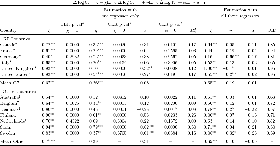
Table 1 summarizes the baseline estimation results for four
alternative econometric specifications nested in equation
(5).
The left panel reports the results from univariate regressions in which
each right-hand side variable enters the estimated specification as
the only regressor. The first column presents the IV estimates of
consumption persistence  , which are for all countries much higher
than the (unreported) OLS estimates and are always highly statistically
significant.
The IV estimates of consumption persistence in table 1 are on average about
0.7—a strong rejection of the random walk proposition which implies a
coefficient of zero. The second column reports p values of the null hypothesis
, which are for all countries much higher
than the (unreported) OLS estimates and are always highly statistically
significant.
The IV estimates of consumption persistence in table 1 are on average about
0.7—a strong rejection of the random walk proposition which implies a
coefficient of zero. The second column reports p values of the null hypothesis
 implied by the heteroscedasticity and autocorrelation robust version of
the conditional likelihood ratio (HAR-CLR) test of Andrews, Moreira, and
Stock (2004). The test is robust to potentially weak instruments and is
effectively uniformly most powerful among tests invariant to rotations of the
instruments. The
implied by the heteroscedasticity and autocorrelation robust version of
the conditional likelihood ratio (HAR-CLR) test of Andrews, Moreira, and
Stock (2004). The test is robust to potentially weak instruments and is
effectively uniformly most powerful among tests invariant to rotations of the
instruments. The  values indicate that the zero restriction on
  is soundly
rejected in almost all countries.
is soundly
rejected in almost all countries.
The third column estimates the Campbell–Mankiw model. Our results
are broadly consistent with the evidence presented in Campbell and
Mankiw (1991): Rule-of-thumb consumers (for whom, by assumption,
consumption equals current income) are on average estimated to earn about
 of aggregate income. Interestingly, the estimates of
  in the left
panel are often less significant than those of consumption persistence
in the left
panel are often less significant than those of consumption persistence  and are in three or four cases insignificant (depending on whether the
standard or HAR-CLR p values are used). This means that—aside from the
question of how the Campbell–Mankiw model stands up against the
alternative of habit formation or sticky expectations—rule-of-thumb spending
behavior cannot be reliably detected in about a third of our sample
countries.
and are in three or four cases insignificant (depending on whether the
standard or HAR-CLR p values are used). This means that—aside from the
question of how the Campbell–Mankiw model stands up against the
alternative of habit formation or sticky expectations—rule-of-thumb spending
behavior cannot be reliably detected in about a third of our sample
countries.
The fifth column investigates the relative importance of wealth (expressed as
the ratio of net financial assets to income) in aggregate consumption dynamics.
The coefficient on the wealth–to–income ratio,  , turns out to be statistically
significant only in four countries, although the HAR-CLR
, turns out to be statistically
significant only in four countries, although the HAR-CLR  values suggest
more often that
values suggest
more often that  is not zero. In addition, the coefficient
  has in most
countries the opposite sign to that predicted by either precautionary saving
theory or intertemporal substitution as channelled through the interest rate.
This is unsurprising for at least two reasons. First, the overwhelming significance
of consumption (and also income) in the previous regressions implies a severe
omitted-variable bias problem with the univariate regression that only includes
wealth. Second, the previous literature generally finds little evidence of interest
rate or precautionary saving effects in aggregate consumption growth
data.
has in most
countries the opposite sign to that predicted by either precautionary saving
theory or intertemporal substitution as channelled through the interest rate.
This is unsurprising for at least two reasons. First, the overwhelming significance
of consumption (and also income) in the previous regressions implies a severe
omitted-variable bias problem with the univariate regression that only includes
wealth. Second, the previous literature generally finds little evidence of interest
rate or precautionary saving effects in aggregate consumption growth
data.
The last column of the left panel displays the adjusted  s from the
first-stage regressions of consumption growth on instruments (denoted
s from the
first-stage regressions of consumption growth on instruments (denoted  ).
This measure of the strength of instruments ranges between 0.1 and 0.2 for most
countries.
).
This measure of the strength of instruments ranges between 0.1 and 0.2 for most
countries. 
The right panel of table 1 reports estimation results when all three regressors
are included in equation (5). The results strongly suggest that past consumption
growth is by far the strongest predictor of current consumption growth. The
average persistence parameter in the country regressions falls only very slightly
compared with the average estimates from univariate regressions reported in the
left panel (from  to
to  ) and remains statistically significant at
the five percent level in ten of our thirteen countries. The predicted income
growth term dominates the lagged consumption term only in one country,
Germany.
The last column of the right panel reports the p-values of the Hansen’s
overidentification test—results of which imply that the null of instrument
exogeneity cannot be rejected.
) and remains statistically significant at
the five percent level in ten of our thirteen countries. The predicted income
growth term dominates the lagged consumption term only in one country,
Germany.
The last column of the right panel reports the p-values of the Hansen’s
overidentification test—results of which imply that the null of instrument
exogeneity cannot be rejected.
Table 2 averages the coefficient estimates from table 1 across various country
groups. As in table 1, while the average consumption persistence  falls
relatively little after income and wealth are added to the estimated equations
(compare the right and left panels of the table), the income and wealth
coefficients become essentially zero. The result holds for all five groups of
countries reported in the table which suggests considerable homogeneity in
falls
relatively little after income and wealth are added to the estimated equations
(compare the right and left panels of the table), the income and wealth
coefficients become essentially zero. The result holds for all five groups of
countries reported in the table which suggests considerable homogeneity in  among advanced economies, a fact already apparent in the previous table with
the results for individual countries.
among advanced economies, a fact already apparent in the previous table with
the results for individual countries.
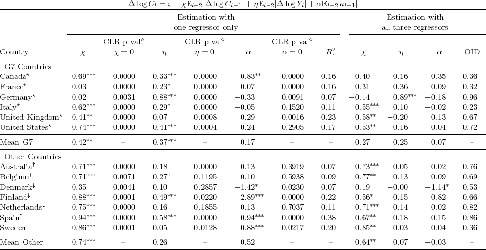
Table 3, whose format is identical to table 1, estimates aggregate consumption
dynamics with an alternative instrument set, in which long-run interest rates and
price volatility have been replaced with income growth and the interest-rate
spread.
The estimation results are broadly consistent with our baseline: (i) the
coefficient on lagged consumption growth in univariate regressions is large and
significant for ten countries, (ii) in the regressions that include all three
regressors, the coefficients on instrumented income growth and wealth
tend to be small and less often statistically significant compared with
univariate regressions, and (iii) lagged consumption growth beats lagged
income in nine horse-race regressions (but gets badly beaten in German
data).
3.2 Kalman Filter/Maximum Likelihood Evidence on Sticky Consumption
Growth
As a more efficient alternative to IV, we also estimate the dynamics of
consumption growth using the Kalman filter. To proceed, it is necessary
to specify an assumption about the stochastic process of measurement
error. We follow the methodology of Sommer (2007) and assume that
measurement error in the log-level of consumption follows an MA(1)
process.
Observed consumption growth,  , can be written as the sum of ‘true’
consumption growth,
, can be written as the sum of ‘true’
consumption growth,  , and a measurement error,
  , as follows:
As noted above,  s are not free parameters but are complicated functions of
 . The Kalman filter jointly estimates the sticky expectations coefficient
  and the degree of the first autocorrelation in measurement errors,
  . The filter
also generates separate estimates of ‘true’ consumption growth,
. The filter
also generates separate estimates of ‘true’ consumption growth,  , and
the measurement error component,
, and
the measurement error component,  . For the purposes of this subsection, we
assume that the correlation structure of measurement error remains unchanged
over the sample period.
. For the purposes of this subsection, we
assume that the correlation structure of measurement error remains unchanged
over the sample period.
The model described in equations (7) and (8) has been rewritten in a
state-space form (see appendix B) and estimated using consumption data for the
countries in our dataset (listed in table 5). Table 4 presents the estimation
results. As in the case of the IV estimation, the coefficient reflecting consumption
growth stickiness,  , is large and highly statistically significant in almost
all sample countries. The value of
, is large and highly statistically significant in almost
all sample countries. The value of  typically ranges between 0.6 and
0.8, with only Denmark and the United Kingdom having coefficients
estimated below 0.4. For the United States, the estimated consumption
persistence is about 0.7, which is consistent with previous studies (e.g.
Fuhrer (2000)).
typically ranges between 0.6 and
0.8, with only Denmark and the United Kingdom having coefficients
estimated below 0.4. For the United States, the estimated consumption
persistence is about 0.7, which is consistent with previous studies (e.g.
Fuhrer (2000)).
It is encouraging that the Kalman filter estimates of consumption persistence
tend to be close to the IV estimates. This suggests that stickiness of
consumption growth is a robust feature of the data that appears similarly even
when viewed through quite different lenses.
The estimation results also suggest that measurement error in the level of
consumption is positively and significantly autocorrelated in about half of our
sample countries—a fact that is not surprising given the interpolation techniques
that are often used by statistical agencies when constructing quarterly
consumption data.
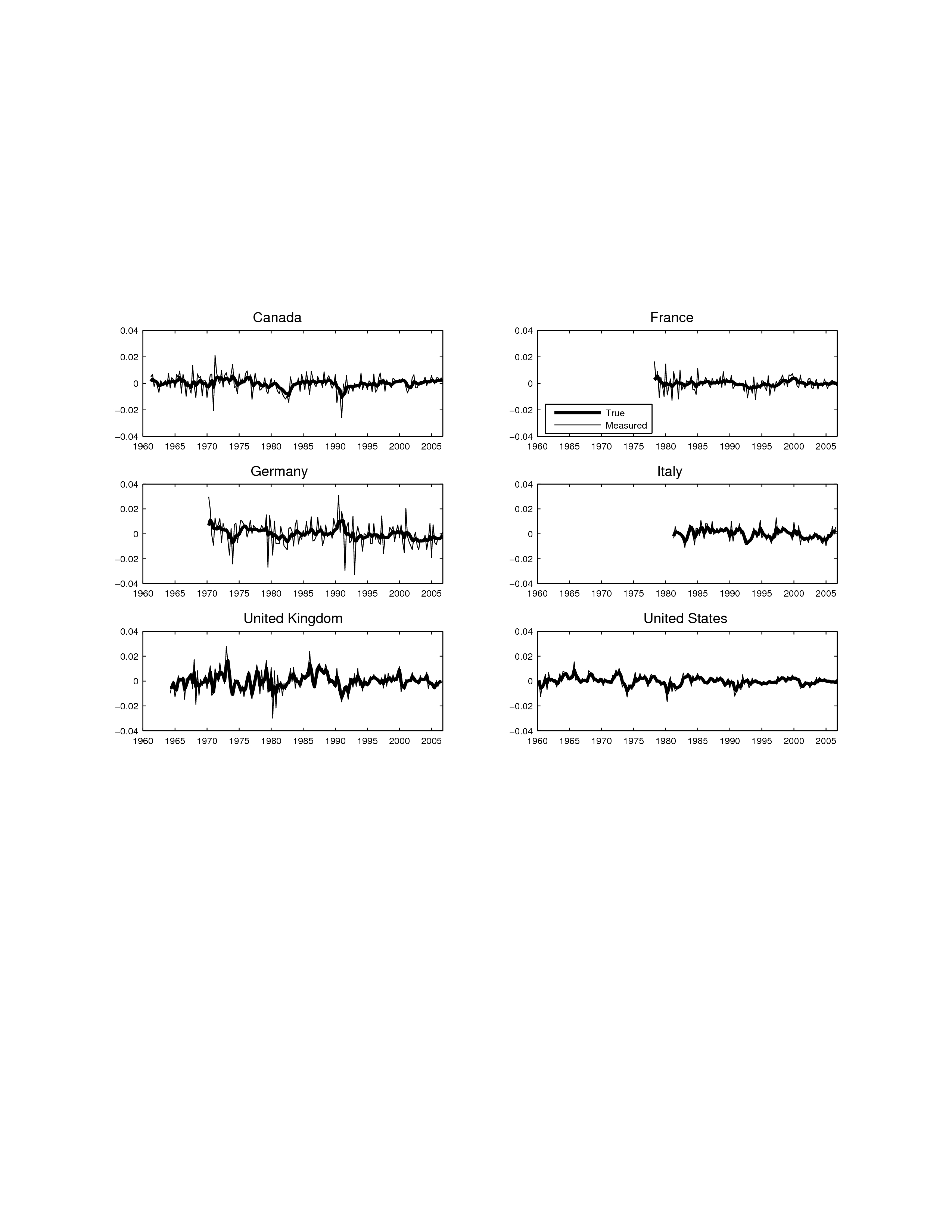
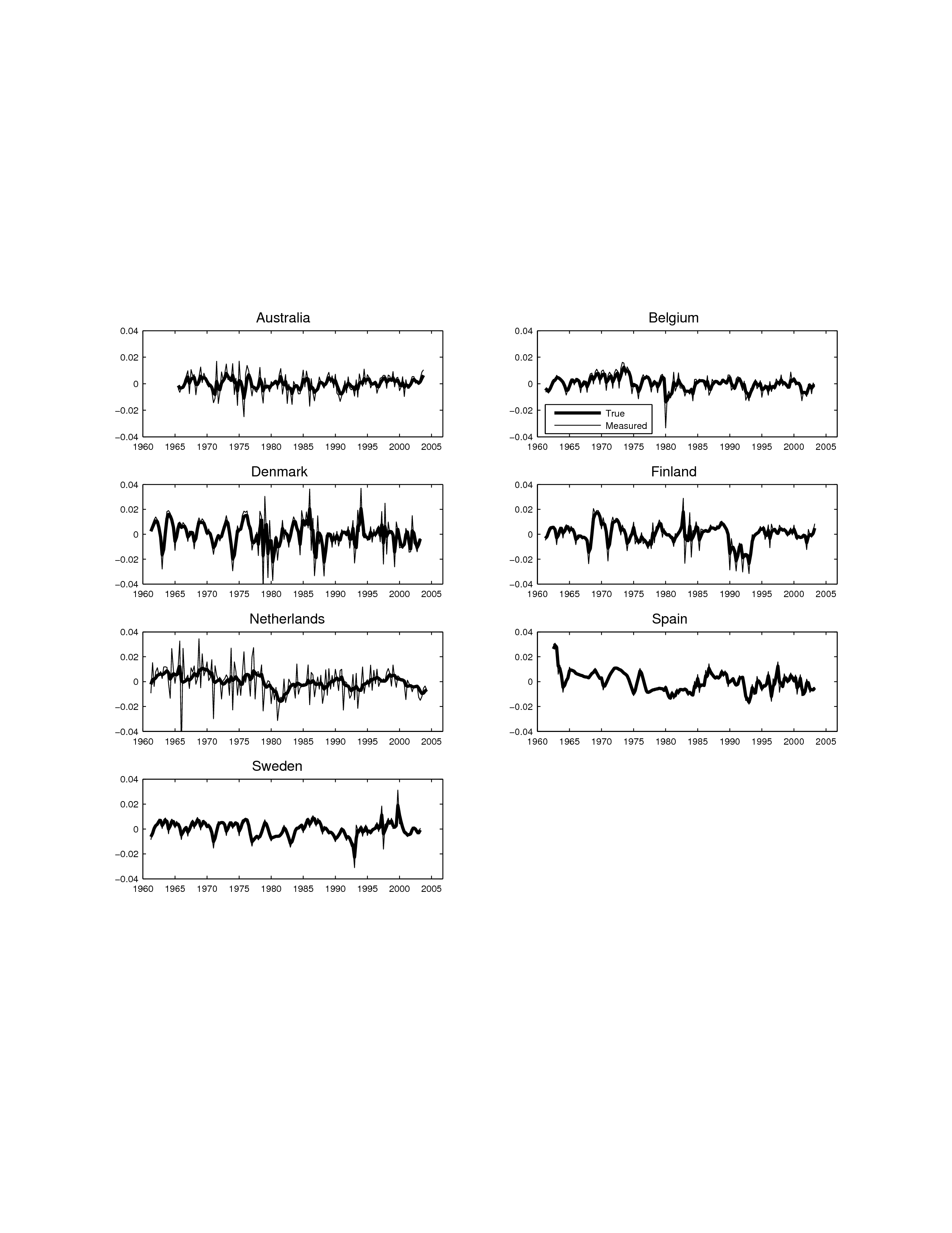
The Kalman filter’s estimate of “true” consumption growth,  , is presented,
along with the raw data, in figures 1 and 2. The Kalman filter estimation suggests
that the share of transitory components in published quarterly consumption data
is large (about 50 percent for the United States and even more for some
countries).
To see how the restrictions on
, is presented,
along with the raw data, in figures 1 and 2. The Kalman filter estimation suggests
that the share of transitory components in published quarterly consumption data
is large (about 50 percent for the United States and even more for some
countries).
To see how the restrictions on  s imposed by the theoretical model with habits
affect estimates of
s imposed by the theoretical model with habits
affect estimates of  , we have also experimented with several versions of model
(7)–(8) in which
, we have also experimented with several versions of model
(7)–(8) in which  s are free parameters (rather than known functions of
  ). In
such models, consumption sluggishness
). In
such models, consumption sluggishness  robustly turns out to be similar to
the values shown in Table 4. However, the fact that in a few cases
robustly turns out to be similar to
the values shown in Table 4. However, the fact that in a few cases  s appear
unrealistic (greater than one or smaller than minus one) suggests that
imposing theoretical restrictions is helpful in identifying them (rather than
s appear
unrealistic (greater than one or smaller than minus one) suggests that
imposing theoretical restrictions is helpful in identifying them (rather than
 ).
).
3.2.1 Relationship with the Structural Estimation Literature
The state-space representation (7)–(8) fits nicely into the structural DSGE
framework recently proposed by Ireland (2004), who estimates a small
log-linearized model with the Kalman filter. Control variables  in
his model can be solved in terms of state variables
in
his model can be solved in terms of state variables  and residuals
 :
:
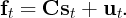 | (9) |
Ireland, p. 1210 views the disturbances  as follows: “the residuals [
 ] may
… soak up both measurement errors, but they can be interpreted more liberally
as capturing all of the movements and co-movements in the data that
the real business cycle model, because of its elegance and simplicity,
cannot explain.” Once we plug our transition equation for consumption
growth (8) into the measurement equation (7), the Kalman filter model
we estimate above has exactly the structure (9) with
] may
… soak up both measurement errors, but they can be interpreted more liberally
as capturing all of the movements and co-movements in the data that
the real business cycle model, because of its elegance and simplicity,
cannot explain.” Once we plug our transition equation for consumption
growth (8) into the measurement equation (7), the Kalman filter model
we estimate above has exactly the structure (9) with  ,
,
 ,
,  and
and  .
.
Thus the state-space representation (7)–(8) can be interpreted as a
stripped-down version of Ireland’s model with consumption habits in which
measured consumption is affected by a combination of measurement errors  and shocks
  to “true” consumption
  . As our main goal is to estimate
consumption stickiness
. As our main goal is to estimate
consumption stickiness  , we do not take a stand on where the consumption
shocks
, we do not take a stand on where the consumption
shocks  come from (be it news about income, wealth, interest rates, fiscal
policy or something else). Our model is simple enough to be estimable using
classical techniques, including the maximum likelihood estimator, so that data
have complete control over the estimates of
come from (be it news about income, wealth, interest rates, fiscal
policy or something else). Our model is simple enough to be estimable using
classical techniques, including the maximum likelihood estimator, so that data
have complete control over the estimates of  , in contrast to larger-scale DSGE
models, which are often inevitably estimated with Bayesian methods with
informative priors.
, in contrast to larger-scale DSGE
models, which are often inevitably estimated with Bayesian methods with
informative priors.
4 Conclusions
Hall (1978) provided macroeconomists with a clean theoretical benchmark to
which actual consumption data could be compared: Consumption growth should
be essentially unpredictable. In contrast with this benchmark, we find that, when
econometric techniques that account for measurement error are used,
consumption growth exhibits a high degree of persistence or “momentum.” The
stickiness of aggregate consumption growth can be interpreted as reflecting the
behavior of fully informed households with a strong consumption habit, or the
behavior of an aggregate economy in which households are not always perfectly
up to date in their knowledge of macroeconomic developments. Fitting the model
to data from thirteen countries, we estimate that consumption growth
persistence is always significantly above the random-walk benchmark of 0 and is
never robustly different from about 0.7. Our analysis also suggests that, on
balance, the model of sticky consumption growth describes aggregate
consumption data better than the rule-of-thumb model of Campbell and
Mankiw (1989), although our point estimates do typically indicate that a
modest proportion of aggregate income (in the range of 10–20 percent)
may be received by households who consume their current income every
quarter.
Our findings imply that the large literature claiming to find evidence of sticky
consumption growth in the U.S. probably cannot be explained away as reflecting
time aggregation problems or other mistreatment of the data, suggesting that
many of the insights gleaned from that literature are likely applicable to other
countries as well. (However, it is worth bearing in mind that analyses that rely
heavily on the literal interpretation of the habits-in-the-utility-function
framework, such as calculations of the welfare cost of aggregate fluctuations, may
not hold up under alternative interpretations of consumption growth
stickiness.)
Our analysis also strengthens a key policy message about the sluggish average
response of consumption to monetary and fiscal policy innovations highlighted
earlier in the context of the habit formation literature—an important policy
consideration at the current cyclical juncture in many countries, including in the
United States.
Table 2: Consumption Dynamics—Groups of Countries (Simple Averages)
Notes: Instruments: Lags  and
and  of the unemployment rate, long-run interest rate, price volatility and consumer
sentiment. Left Panel: Regressions were estimated with one regressor only. Right Panel: Regressions were estimated with all three
regressors. Robust standard errors are in parentheses.
of the unemployment rate, long-run interest rate, price volatility and consumer
sentiment. Left Panel: Regressions were estimated with one regressor only. Right Panel: Regressions were estimated with all three
regressors. Robust standard errors are in parentheses.  Statistical significance at
  percent. Standard errors
are simple averages of individual countries in a given group.
percent. Standard errors
are simple averages of individual countries in a given group.
All countries: Canada, France, Germany, Italy, the United Kingdom, the United States, Australia, Belgium, Denmark, Finland, the
Netherlands, Spain, Sweden. G7 countries: Canada, France, Germany, Italy, the United Kingdom, the United States. Anglo–Saxon
Countries: Australia, Canada, the United Kingdom, the United States. Euro Area Countries: France, Germany, Italy, Belgium,
Finland, the Netherlands, Spain. European Union: France, Germany, Italy, the United Kingdom, Belgium, Denmark, Finland, the
Netherlands, Spain, Sweden.
Appendix A: Description of Data
Data for the G-7 economies are from the Haver Analytics database. Data for other countries are from
the database of the NiGEM model of the NIESR Institute, London. The original sources for most of
these data are OECD, Eurostat, national statistical offices and central banks. Income is measured as
personal disposable income. Wealth is approximated using data on the net financial wealth. All series
were deflated with consumption deflators and expressed in per capita terms. The population series are
from DRI International and were interpolated from annual data to quarterly observations.
Japan is not included in our sample as creating a quarterly dataset with consumption
data going prior to 1980 would involve splicing consumption series based on three very
different methodologies. Adjustments to the Japanese national accounts methodology in 2002
and 2004 have significantly improved the reliability of quarterly consumption series but
the current-methodology data are only available since Q1:1994 (International Monetary
Fund (2006)).
We thank Roberto Golinelli for consumer sentiment series for G7 countries and Australia used
(and described in detail) in Golinelli and Parigi (2004). (We have not used consumer
sentiment series for the remaining countries, because the data are not available before
1985.) We are grateful to Carol Bertaut and Nathalie Girouard for providing us with the
data used in Bertaut (2002) and Catte, Girouard, Price, and Andre (2004), respectively.
Ray Barrell, Amanda Choy and Robert Metz answered our questions about the NiGEM’s
database.
Table 5: Consumption Data, Its Sources, and Samples for IV Regressions
| Country | Time Frame | Consumption/Source | Income/Source | Wealth/Source |
| G7 Countries
|
| Canada | Q4:1970–Q3:2002 | NDS/Haver | PDI/Haver | NFW/NiGEM |
| France | Q1:1985–Q4:2003 | NDS/Haver | PDI/Haver | NFW/NiGEM |
Germany | Q4:1975–Q4:2002 | NDS/Haver | PDI/Haver | NFW/NiGEM |
| Italy | Q1:1981–Q4:2003 | NDS/Haver | PDI/Haver | NFW/NiGEM |
| United Kingdom | Q1:1974–Q4:2003 | NDS/Haver | PDI/Haver | NFW/NiGEM |
| United States | Q3:1962–Q2:2004 | NDS/Haver | PDI/Haver | NFW/NiGEM |
| Other Countries
|
| Australia | Q4:1975–Q4:1999 | PCE/Haver | PDI/Haver | NFW/NiGEM |
| Belgium | Q2:1980–Q4:2002 | PCE/NiGEM&MEI | PDI/NiGEM&MEI | NFW/NiGEM |
| Denmark | Q1:1977–Q2:2003 | PCE/NiGEM&MEI | PDI/NiGEM&MEI | NFW/NiGEM |
| Finland | Q3:1973–Q2:2003 | PCE/NiGEM&MEI | PDI/NiGEM&MEI | NFW/NiGEM |
| Netherlands | Q1:1975–Q4:2002 | PCE/NiGEM&MEI | PDI/NiGEM&MEI | NFW/NiGEM |
| Spain | Q1:1978–Q4:1999 | PCE/NiGEM&MEI | PDI/NiGEM&MEI | NFW/NiGEM |
| Sweden | Q1:1977–Q4:2002 | PCE/NiGEM&MEI | PDI/NiGEM&MEI | NFW/NiGEM |
| |
Notes: PCE Total personal consumption expenditures, NDS
 Nondurables and services, PDI
 Personal disposable
income, NFW
Personal disposable
income, NFW Net financial wealth,
  : Regressions for Germany were estimated with a reunification dummy in Q1:1991;
Source: Haver—Haver Analytics, NiGEM—Database of the NiGEM model of the NIESR Institute, London, MEI—Main Economic
Indicators of OECD.
: Regressions for Germany were estimated with a reunification dummy in Q1:1991;
Source: Haver—Haver Analytics, NiGEM—Database of the NiGEM model of the NIESR Institute, London, MEI—Main Economic
Indicators of OECD.
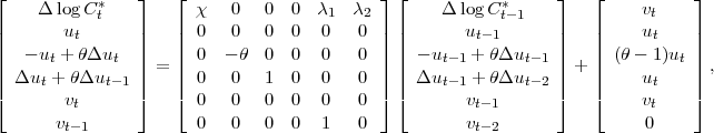
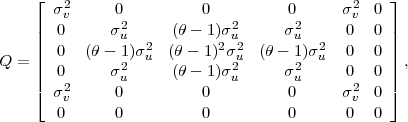
Appendix B: Details of the Kalman Filter Estimation
Following Sommer (2007), equations (7) and (8) can be rewritten in the state-space form with the
measurement equation:
and the state-evolution equation:
and with the associated covariance matrices  and
and
respectively.
The state-space form is estimated with the Kalman filter using the consumption series described in
table 5. The coefficients  and
and  are not free parameters but instead depend on the consumption
persistence coefficient
are not free parameters but instead depend on the consumption
persistence coefficient  :
:  . Our Kalman filter estimation incorporates this
relationship between
. Our Kalman filter estimation incorporates this
relationship between  ,
,  , and
, and  .
.
Figures 1 and 2 display the measured consumption growth  and true consumption
 estimated using the Kalman smoother based on the above state-space model.
References
AKERLOF, GEORGE A., AND JANET L. YELLEN (1985): “A Near-Rational Model of the
Business Cycle, with Wage and Price Intertia,” The Quarterly Journal of Economics, 100(5),
823–38.
AN, SUNGBAE, AND FRANK SCHORFHEIDE (2007): “Bayesian Analysis of DSGE Models,”
Econometric Reviews, 2–4(26), 113–172.
ANDREWS, DONALD W. K., MARCELO MOREIRA, AND JAMES H. STOCK (2004):
“Optimal Invariant Similar Tests for Instrumental Variables Regression,” technical working
paper 299, NBER.
ARUOBA, S. BORAGAN (2008): “Data Revisions Are Not Well Behaved,” Journal of Money,
Credit, and Banking, 40(2-3), 319–340.
BERTAUT, CAROL C. (2002): “Equity Prices, Household Wealth, and Consumption Growth
in Foreign Industrial Countries: Wealth Effects in the 1990s,” Board of Governors of the
Federal Reserve System International Finance Discussion Papers 724.
BRAUN, PHILIP A., GEORGE M. CONSTANTINIDES, AND WAYNE E. FERSON (1993):
“Time Nonseparability in Aggregate Consumption: International Evidence,” European
Economic Review, 37, 897–920.
BUREAU OF ECONOMIC ANALYSIS (2006): “Updated Summary NIPA Methodologies,”
Survey of Current Business, November, Bureau of Economic Analysis, available at
http://www.bea.gov/scb/pdf/2006/11November/1106_nipa_method.pdf.
CALVO, GUILLERMO A. (1983): “Staggered Contracts in a Utility-Maximizing Framework,”
Journal of Monetary Economics, 12, 383–98.
CAMPBELL, JOHN Y., AND ANGUS S. DEATON (1989):
“Why Is Consumption So Smooth?,” Review of Economic Studies, 56, 357–74, Available at
http://ideas.repec.org/a/bla/restud/v56y1989i3p357-73.html.
CAMPBELL, JOHN Y., AND N. GREGORY MANKIW (1989): “Consumption, Income and
Interest Rates: Reinterpreting the Time Series Evidence,” in NBER Macroeconomics Annual,
ed. by Olivier J. Blanchard, and Stanley Fischer, Cambridge, MA. MIT Press.
__________ (1991): “The Response of Consumption to Income: A Cross-Country
Investigation,” European Economic Review, 35(4), 723–756.
CAMPBELL, JOHN Y., AND JOHN H. COCHRANE (1999): “By Force of Habit: A
Consumption-Based Explanation of Aggregate Stock Market Behavior,” Journal of Political
Economy, 107(2), 205–251.
CARROLL, CHRISTOPHER D. (2003): “Macroeconomic Expectations of Households
and Professional Forecasters,” Quarterly Journal of Economics, 118(1), 269–298, At
http://www.econ2.jhu.edu/people/ccarroll/epidemiologyQJE.pdf.
CARROLL, CHRISTOPHER D., JEFFREY C. FUHRER, AND DAVID W. WILCOX (1994):
“Does Consumer Sentiment Forecast Household Spending? If So, Why?,” American Economic
Review, 84(5), 1397–1408.
CARROLL, CHRISTOPHER D., JODY R. OVERLAND, AND DAVID N. WEIL (1997):
“Comparison Utility in a Growth Model,” Journal of Economic Growth, 2(4), 339–367,
Available at http://www.econ2.jhu.edu/people/ccarroll/compare.pdf.
__________ (2000): “Saving and Growth with Habit Formation,” American Economic Review,
90(3), 341–355, Available at http://www.econ2.jhu.edu/people/ccarroll/AERHabits.pdf.
CARROLL, CHRISTOPHER D., AND ANDREW A. SAMWICK (1997): “The Nature of
Precautionary Wealth,” Journal of Monetary Economics, 40(1), 41–71, Available at
http://www.econ2.jhu.edu/people/ccarroll/nature.pdf.
CARROLL, CHRISTOPHER D., AND JIRI SLACALEK (2007): “Sticky Expectations and
Consumption Dynamics,” Manuscript, Johns Hopkins University.
CATTE, PIETRO, NATHALIE GIROUARD, ROBERT PRICE, AND CHRISTOPHE ANDRE
(2004): “Housing Markets, Wealth and the Business Cycle,” OECD Economics Department
Working Papers 394, OECD.
COCHRANE, JOHN H. (1991): “The Sensitivity of Tests of the Intertemporal Allocation of
Consumption to Near-Rational Alternatives,” American Economic Review, 79, 319–37.
CONSTANTINIDES, GEORGE M. (1990): “Habit Formation: A Resolution of the Equity
Premium Puzzle,” Journal of Political Economy, 98, 519–43.
DYNAN, KAREN E. (2000): “Habit Formation in Consumer Preferences: Evidence from
Panel Data,” American Economic Review, 90(3).
FERSON, WAYNE E., AND GEORGE M. CONSTANTINIDES (1991): “Habit Persistence and
Durability in Aggregate Consumption: Empirical Tests,” Journal of Financial Economics,
29(2), 199–240.
FLAVIN, MARJORIE B. (1981): “The Adjustment of Consumption to Changing
Expectations About Future Income,” Journal of Political Economy, 89, 974–1009, Available
at http://ideas.repec.org/a/ucp/jpolec/v89y1981i5p974-1009.html.
FRIEDMAN, MILTON A. (1957): A Theory of the Consumption Function. Princeton
University Press.
FUCHS-SCHüNDELN, NICOLA, AND MATTHIAS SCHüNDELN (2005): “Precautionary Savings
and Self-Selection: Evidence from the German Reunification “Experiment”,” Quarterly
Journal of Economics, 120(3), 1085–1120.
FUHRER, JEFFREY C. (2000): “Habit Formation in Consumption and Its Implication for
Monetary-Policy Models,” American Economic Review, 90(3), 367–390.
GOLINELLI, ROBERTO, AND GIUSEPPE PARIGI (2004): “Consumer Sentiment and Economic
Activity: A Cross Country Comparison,” Journal of Business Cycle Measurement and
Analysis, 1(2), 147–170.
GOURINCHAS, PIERRE-OLIVIER, AND JONATHAN PARKER (2002): “Consumption Over the
Life Cycle,” Econometrica, 70(1), 47–89.
GRUBER, JOSEPH W. (2004): “A Present Value Test of Habits and the Current Account,”
Journal of Monetary Economics, 51(7), 1495–1507.
HALL, ROBERT E. (1978): “Stochastic Implications of the Life-Cycle/Permanent Income
Hypothesis: Theory and Evidence,” Journal of Political Economy, 96, 971–87, Available at
http://www.stanford.edu/~rehall/Stochastic-JPE-Dec-1978.pdf.
__________ (1988): “Intertemporal
Substitution in Consumption,” Journal of Political Economy, XCVI, 339–357, Available at
http://www.stanford.edu/~rehall/Intertemporal-JPE-April-1988.pdf.
INTERNATIONAL MONETARY FUND (2006): “Japan: Report on the Observance of Standards
and Codes—Data Module, Response by the Authorities, and Detailed Assessments Using the
Data Quality Assessment Framework (DQAF),” IMF Country Report 06/115, International
Monetary Fund, March.
IRELAND, PETER N. (2004): “A Method for Taking Models to the Data,” Journal of
Economic Dynamics and Control, 28, 1205–1226.
LETTAU, MARTIN, AND SYDNEY LUDVIGSON (2004): “Understanding Trend and Cycle in
Asset Values: Reevaluating the Wealth Effect on Consumption,” American Economic Review,
94(1), 276–299.
LJUNGQVIST, LARS, AND HARALD UHLIG (2000): “Tax Policy and Aggregate Demand
Management under Catching Up with the Joneses,” American Economic Review, 90(3),
356–366.
LUDVIGSON, SYDNEY, AND MARTIN LETTAU (2001): “Consumption, Aggregate Wealth,
and Expected Stock Returns,” Journal of Finance, 56(3), 815–49.
LUDVIGSON, SYDNEY, AND ALEXANDER MICHAELIDES (2001): “Does Buffer Stock Saving
Explain the Smoothness and Excess Sensitivity of Consumption?,” American Economic
Review, 91(3), 631–647.
LUENGO-PRADO, MARíA JOSé, AND BENT E. SØRENSEN (2008): “What Can Explain
Excess Smoothness and Sensitivity of State-Level Consumption?,” The Review of Economics
and Statistics, 90(1), 65–80.
MANKIW, N. GREGORY (1982): “Hall’s Consumption Hypothesis and Durable Goods,”
Journal of Monetary Economics, 10(3), 417–425.
MANKIW, N. GREGORY, AND RICARDO REIS (2001): “Sticky Information Versus Sticky
Prices: A Proposal to Replace the New Keynesian Phillips Curve,” Quarterly Journal of
Economics, 117(4), 1295–1328.
MICHAELIDES, ALEXANDER (2002): “Buffer Stock Saving and Habit Formation,”
Manuscript, London School of Economics.
MUELLBAUER, JOHN (1988): “Habits, Rationality and Myopia in the Life Cycle
Consumption Function,” Annales d’Economie et de Statistique, 9, 47–70.
OKUN, ARTHUR M. (1981): Prices and Quantities: A Macroeconomic Analysis. Brookings
Institution Press.
PISCHKE, JöRN-STEFFEN (1995): “Individual Income, Incomplete Information, and
Aggregate Consumption,” Econometrica, 63(4), 805–40.
REIS, RICARDO (2006): “Inattentive Consumers,” Journal of Monetary Economics, 53(8),
1761–1800.
SHORE, STEPHEN H., AND JOSHUA S. WHITE (2006): “External Habit Formation and
the Home Bias Puzzle,” working paper, The Wharton School, University of Pennsylvania.
SIMS, CHRISTOPHER A. (2003):
“Implications of Rational Inattention,” Journal of Monetary Economics, 50(3), 665–690,
available at http://ideas.repec.org/a/eee/moneco/v50y2003i3p665-690.html.
SMETS, FRANK, AND RAF WOUTERS (2003): “An Estimated Dynamic Stochastic General
Equilibrium Model of the Euro Area,” Journal of European Economic Association, 5(1),
1123–1175.
SOMMER, MARTIN (2007): “Habit Formation and Aggregate Consumption Dynamics,” The
B.E. Journal of Macroeconomics—Advances, 7(1), Article 21.
VISSING-JØRGENSEN, ANNETTE (2002): “Limited Asset Market Participation and the
Elasticity of Intertemporal Substitution,” Journal of Political Economy, 110(825–53),
339–357.
WILCOX, DAVID W. (1992): “The Construction of the U.S. Consumption Data: Some Facts
and Their Implications for Empirical Research,” American Economic Review, 82(4), 922–941.
WORKING, HOLBROOK (1960): “Note on the Correlation of First Differences of Averages in
a Random Chain,” Econometrica, 28(4), 916–18.

![Δ logCt = ς + χEt-2[Δ logCt-1]+ η Et- 2[Δ logYt]+ α Et-2[at-1]](cssIntlStickyC128x.png)


![Δ log C = ς + χ E [Δ log C ] + ηE [Δ log Y ] + αE [a ]
t t-2 t- 1 t-2 t t-2 t-1](cssIntlStickyC808x.png)


![Δ log Ct = ς + χEt- 2[Δ logCt- 1]+ ηEt-2[Δ log Yt]+ αEt-2[at- 1]](cssIntlStickyC1059x.png)


![⌊ * ⌋
Δ log Ct
|| ut ||
Δ logC = c + [100100 ]|| - ut + θΔut || + 0,
t 0 || Δut + θΔut -1 ||
⌈ vt ⌉
vt- 1](cssIntlStickyC2028x.png)