 is to maximize expected
discounted utility from consumption over the remainder of a lifetime that ends in period
is to maximize expected
discounted utility from consumption over the remainder of a lifetime that ends in period  :
:
SolvingMicroDSOPs, April 7, 2022
Note: The code associated with this document should work (though the Matlab code may be out of date), but has been superceded by the set of tools available in the Econ-ARK toolkit, more specifically the HARK Framework. The SMM estination code at the end has specifically been superceded by the SolvingMicroDSOPs REMARK
_____________________________________________________________________________________
Abstract
These notes describe tools for solving microeconomic dynamic stochastic optimization problems,
and show how to use those tools for efficiently estimating a standard life cycle consumption/saving
model using microeconomic data. No attempt is made at a systematic overview of the many possible
technical choices; instead, I present a specific set of methods that have proven useful in my own work
(and explain why other popular methods, such as value function iteration, are a bad idea). Paired
with these notes is Mathematica, Matlab, and Python software that solves the problems described in
the text.
Dynamic Stochastic Optimization, Method of Simulated Moments, Structural Estimation
E21, F41
| PDF: | https://github.com/llorracc/SolvingMicroDSOPs/blob/master/SolvingMicroDSOPs.pdf |
| Slides: | https://github.com/llorracc/SolvingMicroDSOPs/blob/master/SolvingMicroDSOPs-Slides.pdf |
| Web: | https://llorracc.github.io/SolvingMicroDSOPs |
| Code: | https://github.com/llorracc/SolvingMicroDSOPs/tree/master/Code |
| Archive: | https://github.com/llorracc/SolvingMicroDSOPs |
| (Contains LaTeX code for this document and software producing figures and results) |
1Carroll: Department of Economics, Johns Hopkins University, Baltimore, MD, http://www.econ2.jhu.edu/people/ccarroll/, ccarroll@jhu.edu, Phone: (410) 516-7602 The notes were originally written for my Advanced Topics in Macroeconomic Theory class at Johns Hopkins University; instructors elsewhere are welcome to use them for teaching purposes. Relative to earlier drafts, this version incorporates several improvements related to new results in the paper “Theoretical Foundations of Buffer Stock Saving” (especially tools for approximating the consumption and value functions). Like the last major draft, it also builds on material in “The Method of Endogenous Gridpoints for Solving Dynamic Stochastic Optimization Problems” published in Economics Letters, available at http://www.econ2.jhu.edu/people/ccarroll/EndogenousArchive.zip, and by including sample code for a method of simulated moments estimation of the life cycle model a la Gourinchas and Parker (2002) and Cagetti (2003). Background derivations, notation, and related subjects are treated in my class notes for first year macro, available at http://www.econ2.jhu.edu/people/ccarroll/public/lecturenotes/consumption. I am grateful to several generations of graduate students in helping me to refine these notes, to Marc Chan for help in updating the text and software to be consistent with Carroll (2006), to Kiichi Tokuoka for drafting the section on structural estimation, to Damiano Sandri for exceptionally insightful help in revising and updating the method of simulated moments estimation section, and to Weifeng Wu and Metin Uyanik for revising to be consistent with the ‘method of moderation’ and other improvements. All errors are my own.
Calculating the mathematically optimal amount to save is a remarkably difficult problem. Under well-founded assumptions about the nature of risk (and attitudes toward risk), the problem cannot be solved analytically; computational solutions are the only option. To avoid having to solve this hard problem, past generations of economists showed impressive ingenuity in reformulating the question. Budding graduate students are still taught a host of tricks whose purpose is partly to avoid the resort to numerical solutions: Quadratic or Constant Absolute Risk Aversion utility, perfect markets, perfect insurance, perfect foresight, the “timeless” perspective, the restriction of uncertainty to very special kinds,1 and more.
The motivation is mainly to exchange an intractable general problem for a tractable specific alternative. Unfortunately, the burgeoning literature on numerical solutions has shown that the features that yield tractability also profoundly change the solution. These tricks are excuses to solve a problem that has defined away the central difficulty: Understanding the proper role of uncertainty (and other complexities like constraints) in optimal intertemporal choice.
The temptation to use such tricks (and the tolerance for them in leading academic journals) is palpably lessening, thanks to advances in mathematical analysis, increasing computing power, and the growing capabilities of numerical computation software. Together, such tools permit today’s laptop computers to solve problems that required supercomputers a decade ago (and, before that, could not be solved at all).
These points are not unique to the consumption/saving problem; the same propositions apply to almost any question that involves both intertemporal choice and uncertainty, including many aspects of the behavior of firms and governments.
Given the ubiquity of such problems, one might expect that the use of numerical methods for solving dynamic optimization problems would by now be nearly as common as the use of econometric methods in empirical work.
Of course, we remain far from that equilibrium. The most plausible explanation for the gap is that barriers to the use of numerical methods have remained forbiddingly high.
These lecture notes provide a gentle introduction to a particular set of solution tools and show how they can be used to solve some canonical problems in consumption choice and portfolio allocation. Specifically, the notes describe and solve optimization problems for a consumer facing uninsurable idiosyncratic risk to nonfinancial income (e.g., labor or transfer income),2 with detailed intuitive discussion of the various mathematical and computational techniques that, together, speed the solution by many orders of magnitude compared to “brute force” methods. The problem is solved with and without liquidity constraints, and the infinite horizon solution is obtained as the limit of the finite horizon solution. After the basic consumption/saving problem with a deterministic interest rate is described and solved, an extension with portfolio choice between a riskless and a risky asset is also solved. Finally, a simple example is presented of how to use these methods (via the statistical ‘method of simulated moments’ or MSM; sometimes called ‘simulated method of moments’ or SMM) to estimate structural parameters like the coefficient of relative risk aversion (a la Gourinchas and Parker (2002) and Cagetti (2003)).
We are interested in the behavior a consumer whose goal in period is to maximize expected
discounted utility from consumption over the remainder of a lifetime that ends in period :
![[ ]
T∑− t
max 𝔼t βn𝜃𝜃𝜃u(ct+n) ,
n𝜃𝜃𝜃=0](SolvingMicroDSOPs2x.svg) | (1) |
and whose circumstances evolve according to the transition equations3
 | (2) |
where the variables are
 |
For now, we will assume that the exogenous variables evolve as follows:
 |
Using the fact about lognormally distributed variables
ELogNorm4
that if  then
then ![log 𝔼 [φφφ ] = φ + σ2 ∕2
φ](SolvingMicroDSOPs8x.svg) , assumption the assumption about the
distribution of shocks guarantees that
, assumption the assumption about the
distribution of shocks guarantees that ![log 𝔼[𝜃𝜃𝜃] = 0](SolvingMicroDSOPs9x.svg) which means that
which means that ![𝔼 [𝜃𝜃𝜃]](SolvingMicroDSOPs10x.svg) =1 (the mean
value of the transitory shock is 1).
=1 (the mean
value of the transitory shock is 1).
Equation (3) indicates that we are allowing for a predictable average profile of
income growth over the lifetime  (allowing, for example, for typical career wage
paths).5
(allowing, for example, for typical career wage
paths).5
Finally, the utility function is of the Constant Relative Risk Aversion (CRRA), form,
 .
.
As is well known, this problem can be rewritten in recursive (Bellman equation) form
![vvvt(mt, pt) = max u (ct) + 𝔼t[βvvvt+1(mt+1, pt+1)]
ct](SolvingMicroDSOPs13x.svg) | (3) |
subject to the Dynamic Budget Constraint (DBC) (2) given above, where  measures total
expected discounted utility from behaving optimally now and henceforth.
measures total
expected discounted utility from behaving optimally now and henceforth.
The single most powerful method for speeding the solution of such models is to redefine the
problem in a way that reduces the number of state variables (if possible). In the consumption
problem here, the obvious idea is to see whether the problem can be rewritten in terms of the
ratio of various variables to permanent noncapital (‘labor’) income  (henceforth for brevity
referred to simply as ‘permanent income.’)
(henceforth for brevity
referred to simply as ‘permanent income.’)
In the last period of life, there is no future,  , so the optimal plan is to consume
everything, implying that
, so the optimal plan is to consume
everything, implying that
 | (4) |
Now define nonbold variables as the bold variable divided by the level of permanent
income in the same period, so that, for example,  ; and define
 .6
For our CRRA utility function,
.6
For our CRRA utility function,  , so equation (4) can be rewritten
as
, so equation (4) can be rewritten
as
 |
Now define a new optimization problem:
![vt(mt ) = max u(ct) + 𝔼t[βΦΦΦ1 −ρvt+1(mt+1)]
ct t+1
s.t.
at = mt − ct
mt+1 = (R ∕ΦΦΦt+1) at + 𝜃𝜃𝜃t+1
◟--◝◜--◞
≡ ℛt+1](SolvingMicroDSOPs24x.svg) |
The accumulation equation is the normalized version of the transition equation for
 .7
Then it is easy to see that for
.7
Then it is easy to see that for  ,
,
 |
and so on back to all earlier periods. Hence, if we solve the problem (5) which has only a single
state variable  , we can obtain the levels of the value function, consumption, and all other
variables of interest simply by multiplying the results by the appropriate function of
, we can obtain the levels of the value function, consumption, and all other
variables of interest simply by multiplying the results by the appropriate function of  ,
e.g.
,
e.g.  or
or  . We have thus reduced the
problem from two continuous state variables to one (and thereby enormously simplified its
solution).
. We have thus reduced the
problem from two continuous state variables to one (and thereby enormously simplified its
solution).
For some problems it will not be obvious that there is an appropriate ‘normalizing’ variable, but many problems can be normalized if sufficient thought is given. For example, Valencia (2006) shows how a bank’s optimization problem can be normalized by the level of the bank’s productivity.
The first order condition for (5) with respect to  is
is
![u′(c ) = 𝔼 [β ℛ ΦΦΦ1 −ρv′ (m )]
t t t+1 t+1 t+1 t+1
= 𝔼t [βR ΦΦΦt−+ρ1v ′t+1(mt+1 )]](SolvingMicroDSOPs34x.svg) |
and because the Envelope theorem tells us that
![v ′t(mt ) = 𝔼t[βRΦΦΦ −tρ+1v′t+1(mt+1)]](SolvingMicroDSOPs35x.svg) | (5) |
we can substitute the LHS of (5) for the RHS of (5) to get
 | (6) |
and rolling this equation forward one period yields
 | (7) |
while substituting the LHS in equation (5) gives us the Euler equation for consumption
![′ −ρ ′
u (ct) = 𝔼t [βR ΦΦΦ t+1u (ct+1)].](SolvingMicroDSOPs38x.svg) | (8) |
Now note that in equation (7) neither  nor
nor  has any direct effect on
  - only
the difference between them (i.e. unconsumed market resources or ‘assets’
- only
the difference between them (i.e. unconsumed market resources or ‘assets’  )
matters. It is therefore possible (and will turn out to be convenient) to define a
function8
)
matters. It is therefore possible (and will turn out to be convenient) to define a
function8
![𝔳t(at) = 𝔼t[βΦΦΦ1−t+1ρvt+1(ℛt+1at + 𝜃𝜃𝜃t+1)]](SolvingMicroDSOPs43x.svg) | (9) |
that returns the expected  value associated with ending period
  with any given
amount of assets. This definition implies that
with any given
amount of assets. This definition implies that
![𝔳′(a ) = 𝔼 [βR ΦΦΦ− ρv′ (ℛ a + 𝜃𝜃𝜃 )]
t t t t+1 t+1 t+1 t t+1](SolvingMicroDSOPs46x.svg) | (10) |
or, substituting from equation (7),
![′ [ −ρ ′ ]
𝔳t(at) = 𝔼t βRΦΦΦt+1u (ct+1(ℛt+1at + 𝜃𝜃𝜃t+1)) .](SolvingMicroDSOPs47x.svg) | (11) |
Finally, note for future use that the first order condition (5) can now be rewritten as
 | (12) |
The problem in the second-to-last period of life is:
![v (m ) = max u (c ) + β 𝔼 [ΦΦΦ1 −ρv ((m − c )ℛ + 𝜃𝜃𝜃 )],
T−1 T−1 cT−1 T −1 T−1 T T T−1 T− 1 T T](SolvingMicroDSOPs49x.svg) |
and using (1) the fact that  ; (2) the definition of
  ; (3) the definition of the
expectations operator, and (4) the fact that
; (3) the definition of the
expectations operator, and (4) the fact that  is nonstochastic, this becomes
 |
where  is the cumulative distribution function for
  .
.
In principle, the maximization implicitly defines a function  that yields
optimal consumption in period
that yields
optimal consumption in period  for any given level of resources
  . Unfortunately,
however, there is no general analytical solution to this maximization problem, and so for any
given
. Unfortunately,
however, there is no general analytical solution to this maximization problem, and so for any
given  we must use numerical computational tools to find the
  that maximizes
the expression. This is excruciatingly slow because for every potential
that maximizes
the expression. This is excruciatingly slow because for every potential  to be
considered, the integral must be calculated numerically, and numerical integration is very
slow.
to be
considered, the integral must be calculated numerically, and numerical integration is very
slow.
Our first time-saving step is therefore to construct a discrete approximation to the lognormal
distribution that can be used in place of numerical integration. We calculate an  -point
approximation as follows.
-point
approximation as follows.
Define a set of points from  to
to  on the
 ![[0,1]](SolvingMicroDSOPs65x.svg) interval as the elements of the set
interval as the elements of the set
 .9
Call the inverse of the
.9
Call the inverse of the  distribution
  , and define the points
  . Then the
conditional mean of
. Then the
conditional mean of  in each of the intervals numbered 1 to
  is:
is:
![∫ ♯−1
𝜃𝜃𝜃 ≡ 𝔼 [𝜃𝜃𝜃|♯−1 ≤ 𝜃𝜃𝜃 < ♯− 1] = i 𝜗 dℱ (𝜗 ).
i i− 1 i ♯−1
i−1](SolvingMicroDSOPs73x.svg) | (13) |
The method is illustrated in Figure 1. The solid continuous curve represents the “true” CDF
 for a lognormal distribution such that
 ![𝔼[𝜃𝜃𝜃] = 1](SolvingMicroDSOPs75x.svg) ,
,  . The short vertical line
segments represent the
. The short vertical line
segments represent the  equiprobable values of
  which are used to approximate this
distribution.10
which are used to approximate this
distribution.10
Recalling our definition of  , for
, for 
 | (14) |
so we can rewrite the maximization problem as
 | (15) |
Given a particular value of  , a numerical maximization routine can now find the
  that maximizes (15) in a reasonable amount of time. The Mathematica program that solves
exactly this problem is called 2period.m. (The archive also contains parallel Matlab programs,
but these notes will dwell on the specifics of the Mathematica implementation, which is
superior in many respects.)
that maximizes (15) in a reasonable amount of time. The Mathematica program that solves
exactly this problem is called 2period.m. (The archive also contains parallel Matlab programs,
but these notes will dwell on the specifics of the Mathematica implementation, which is
superior in many respects.)
The first thing 2period.m does is to read in the file functions.m which contains
definitions of the consumption and value functions; functions.m also defines the function
SolveAnotherPeriod which, given the existence in memory of a solution for period  ,
solves for period
,
solves for period  .
.
The next step is to run the programs setup_params.m, setup_grids.m, setup_shocks.m,
respectively. setup_params.m sets values for the parameter values like the coefficient of
relative risk aversion. setup_shocks.m calculates the values for the  defined above (and
puts those values, and the (identical) probability associated with each of them, in the vector
variables
defined above (and
puts those values, and the (identical) probability associated with each of them, in the vector
variables  Vals and
  Prob). Finally, setup_grids.m constructs a list of potential values
of cash-on-hand and saving, then puts them in the vector variables mVec = aVec =
Prob). Finally, setup_grids.m constructs a list of potential values
of cash-on-hand and saving, then puts them in the vector variables mVec = aVec =
 respectively. Then 2period.m runs the program setup_lastperiod.m which
defines the elements necessary to determine behavior in the last period, in which
respectively. Then 2period.m runs the program setup_lastperiod.m which
defines the elements necessary to determine behavior in the last period, in which  and
and  .
.
After all the setup, the only remaining step in 2period.m is to invoke SolveAnotherPeriod,
which constructs the solution for period  given the presence of the solution for period
 (constructed by setup_lastperiod.m).
Because we will always be comparing our solution to the perfect foresight solution, we also
construct the variables required to characterize the perfect foresight consumption function in
periods prior to  . In particular, we construct the list yExpPDV (which contains the PDV of
expected income – ‘expected human wealth’), and yMinPDV which contains the minimum possible
discounted value of future income at the beginning of period
. In particular, we construct the list yExpPDV (which contains the PDV of
expected income – ‘expected human wealth’), and yMinPDV which contains the minimum possible
discounted value of future income at the beginning of period  (‘minimum human
wealth’).11
(‘minimum human
wealth’).11
The perfect foresight consumption function is also constructed (setup_PerfectForesightSolution.m).
This program uses the fact that, in Mathematica, functions can be saved as objects using the
commands # and &. The # denotes the argument of the function, while the &, placed at the end
of the function, tells Mathematica that the function should be saved as an object. In the
program, the last period perfect foresight consumption function is saved as an element in the
list  = {(# - 1 + Last[yExpPDV]) Last[
 Min] &}, where Last[yExpPDV]
gives the just-constructed PDV of human wealth at the beginning of
Min] &}, where Last[yExpPDV]
gives the just-constructed PDV of human wealth at the beginning of  (equal to
1, since current income is included in
(equal to
1, since current income is included in  ), and Last[
 Min] gives the perfect
foresight marginal propensity to consume (equal to 1, since it is optimal to spend all
resources in the last period). Since # in the code stands in for what was called
Min] gives the perfect
foresight marginal propensity to consume (equal to 1, since it is optimal to spend all
resources in the last period). Since # in the code stands in for what was called  in
the model, the discounted total wealth is decomposed into discounted non-human
wealth # - 1 and discounted human wealth Last[yExpPDV]. The resulting formula
then corresponds to
in
the model, the discounted total wealth is decomposed into discounted non-human
wealth # - 1 and discounted human wealth Last[yExpPDV]. The resulting formula
then corresponds to  , which translates to
  for
for
 .
.
The infinite horizon perfect foresight marginal propensity to save
 | (16) |
is also defined because it will be useful in a number of derivations.12
The program then constructs behavior for one iteration back from the last period of life by
using the function AddNewPeriodToParamLifeDates. Using the Mathematica command
AppendTo, various existing lists (which characterized the solution for period  ) are redefined
to include an additional element representing the relevant formulas in the second to last period
of life. For example,
) are redefined
to include an additional element representing the relevant formulas in the second to last period
of life. For example,  Min now has two elements. The second element, given by 1/(1 +
Last[
Min now has two elements. The second element, given by 1/(1 +
Last[ ]/Last[
 Min]), is the perfect foresight marginal propensity to consume in
 .13
.13
Next, the program defines a function  [at_] (in functions_stable.m) which is the
exact implementation of (9): It returns the expectation of the value of behaving
optimally in period
[at_] (in functions_stable.m) which is the
exact implementation of (9): It returns the expectation of the value of behaving
optimally in period  given any specific amount of assets at the end of
  ,
,
 .
.
The heart of the program is the next expression (in functions.m). This expression loops over the values of the variable mVec, solving the maximization problem (given in equation (15)):
![max u[c ] + 𝔳 [mVec [[i]]- c]
c](SolvingMicroDSOPs117x.svg) | (17) |
for each of the  values of mVec (henceforth let’s call these points
  ). The
maximization routine returns two values: the maximized value, and the value of
). The
maximization routine returns two values: the maximized value, and the value of  which
yields that maximized value. When the loop (the Table command) is finished, the variable
vAndcList contains two lists, one with the values
which
yields that maximized value. When the loop (the Table command) is finished, the variable
vAndcList contains two lists, one with the values  and the other with the consumption
levels
and the other with the consumption
levels  associated with the
  .
.
Now we use the first of the really convenient built-in features of Mathematica. Given a set of
points on a function (in this case, the consumption function  ), Mathematica can
create an object called an InterpolatingFunction which when applied to an input
), Mathematica can
create an object called an InterpolatingFunction which when applied to an input  will
yield the value of
will
yield the value of  that corresponds to a linear interpolation of the value of
  from the
points in the InterpolatingFunction object. We can therefore define an approximation to
the consumption function
from the
points in the InterpolatingFunction object. We can therefore define an approximation to
the consumption function  which, when called with an
  that is equal to
one of the points in mVec[[i]] returns the associated value of
that is equal to
one of the points in mVec[[i]] returns the associated value of  , and when called with a
value of
, and when called with a
value of  that is not exactly equal to one of the mVec[[i]], returns the value of
 that reflects a linear interpolation between the
  associated with the two
mVec[[i]] points nearest to
associated with the two
mVec[[i]] points nearest to  . Thus if the function is called with
  and the nearest gridpoints are
  and
and  then the value of
 returned by the function would be
  . We can define a
numerical approximation to the value function
. We can define a
numerical approximation to the value function  in an exactly analogous
way.
in an exactly analogous
way.
Figures 2 and 3 show plots of the  and
and  InterpolatingFunctions that are generated
by the program 2PeriodInt.m. While the
InterpolatingFunctions that are generated
by the program 2PeriodInt.m. While the  function looks very smooth, the fact that the
 function is a set of line segments is very evident. This figure provides the beginning of
the intuition for why trying to approximate the value function directly is a bad idea (in this
context).14
function is a set of line segments is very evident. This figure provides the beginning of
the intuition for why trying to approximate the value function directly is a bad idea (in this
context).14
2period.m works well in the sense that it generates a good approximation to the true optimal
consumption function. However, there is a clear inefficiency in the program: Since it uses
equation (15), for every value of  the program must calculate the utility consequences of
various possible choices of
the program must calculate the utility consequences of
various possible choices of  as it searches for the best choice. But for any given
value of
as it searches for the best choice. But for any given
value of  , there is a good chance that the program may end up calculating the
corresponding
, there is a good chance that the program may end up calculating the
corresponding  many times while maximizing utility from different
  ’s. For
example, it is possible that the program will calculate the value of ending the period
with
’s. For
example, it is possible that the program will calculate the value of ending the period
with  dozens of times. It would be much more efficient if the program
could make that calculation once and then merely recall the value when it is needed
again.
dozens of times. It would be much more efficient if the program
could make that calculation once and then merely recall the value when it is needed
again.
This can be achieved using the same interpolation technique used above to construct a
direct numerical approximation to the value function: Define a grid of possible values for
saving at time  ,
,  (aVec in setup_grids.m), designating the specific points
 ; for each of these values of
  , calculate the vector
  as the collection of
points
as the collection of
points  using equation (9); then construct an InterpolatingFunction
object
using equation (9); then construct an InterpolatingFunction
object  from the list of points on the function captured in the
  and
and  vectors.
Thus, we are now interpolating for the function that reveals
the expected value of ending the period with a given amount of
assets.15
The program 2periodIntExp.m solves this problem. Figure 4 compares the true value
function to the InterpolatingFunction approximation; the functions are of course identical
at the gridpoints chosen for  and they appear reasonably close except in the region
below
and they appear reasonably close except in the region
below  .
.
Nevertheless, the resulting consumption rule obtained when  is used instead of
 is surprisingly bad, as shown in figure 5. For example, when
  goes
from 2 to 3,
goes
from 2 to 3,  goes from about 1 to about 2, yet when
  goes from 3 to
4,
goes from 3 to
4,  goes from about 2 to about 2.05. The function fails even to be strictly
concave, which is distressing because Carroll and Kimball (1996) prove that the correct
consumption function is strictly concave in a wide class of problems that includes this
problem.
goes from about 2 to about 2.05. The function fails even to be strictly
concave, which is distressing because Carroll and Kimball (1996) prove that the correct
consumption function is strictly concave in a wide class of problems that includes this
problem.
Loosely speaking, our difficulty reflects the fact that the consumption choice is governed by
the marginal value function, not by the level of the value function (which is the object that we
approximated). To understand this point, recall that a quadratic utility function exhibits risk
aversion because with a stochastic  ,
,
![𝔼 [− (c − /c)2] < − (𝔼[c] − /c)2](SolvingMicroDSOPs177x.svg) | (18) |
where  is the ‘bliss point’. However, unlike the CRRA utility function, with quadratic utility
the consumption/saving behavior of consumers is unaffected by risk since behavior is
determined by the first order condition, which depends on marginal utility, and when utility is
quadratic, marginal utility is unaffected by risk:
is the ‘bliss point’. However, unlike the CRRA utility function, with quadratic utility
the consumption/saving behavior of consumers is unaffected by risk since behavior is
determined by the first order condition, which depends on marginal utility, and when utility is
quadratic, marginal utility is unaffected by risk:
![𝔼[− 2(c − /c)] = − 2(𝔼[c] − /c).](SolvingMicroDSOPs179x.svg) | (19) |
Intuitively, if one’s goal is to accurately capture choices that are governed by marginal value, numerical techniques that approximate the marginal value function will yield a more accurate approximation to optimal behavior than techniques that approximate the level of the value function.
The first order condition of the maximization problem in period  is:
is:
![′ −ρ ′
u (cT −1) = β 𝔼T −1[ΦΦΦ T Ru (cT)]
( 1 ) ∑n𝜃𝜃𝜃
c−T ρ−1 = Rβ --- ΦΦΦ −Tρ(R (mT −1 − cT −1) + 𝜃𝜃𝜃i)−ρ .
n𝜃𝜃𝜃 i=1](SolvingMicroDSOPs181x.svg) | (20) |
The downward-sloping curve in Figure 6 shows the value of  for our baseline
parameter values for
for our baseline
parameter values for  (the horizontal axis). The solid upward-sloping curve
shows the value of the RHS of (20) as a function of
(the horizontal axis). The solid upward-sloping curve
shows the value of the RHS of (20) as a function of  under the assumption that
 . Constructing this figure is rather time-consuming, because for every value of
 plotted we must calculate the RHS of (20). The value of
  for which the RHS and
LHS of (20) are equal is the optimal level of consumption given that
for which the RHS and
LHS of (20) are equal is the optimal level of consumption given that  , so the
intersection of the downward-sloping and the upward-sloping curves gives the optimal value of
, so the
intersection of the downward-sloping and the upward-sloping curves gives the optimal value of
 . As we can see, the two curves intersect just below
  . Similarly, the
upward-sloping dashed curve shows the expected value of the RHS of (20) under the
assumption that
. Similarly, the
upward-sloping dashed curve shows the expected value of the RHS of (20) under the
assumption that  , and the intersection of this curve with
  yields the
optimal level of consumption if
yields the
optimal level of consumption if  . These two curves intersect slightly below
 . Thus, increasing
  from 3 to 4 increases optimal consumption by about
0.5.
from 3 to 4 increases optimal consumption by about
0.5.
Now consider the derivative of our function  . Because we have constructed
 as a linear interpolation, the slope of
  between any two adjacent points
 is constant. The level of the slope immediately below any particular
gridpoint is different, of course, from the slope above that gridpoint, a fact which implies that
the derivative of
is constant. The level of the slope immediately below any particular
gridpoint is different, of course, from the slope above that gridpoint, a fact which implies that
the derivative of  follows a step function.
The solid-line step function in Figure 6 depicts the actual value of  . When
we attempt to find optimal values of
. When
we attempt to find optimal values of  given
given  using
using  , the numerical
optimization routine will return the
, the numerical
optimization routine will return the  for which
  . Thus,
for
. Thus,
for  the program will return the value of
  for which the downward-sloping
 curve intersects with the
  ; as the diagram shows, this value is
exactly equal to 2. Similarly, if we ask the routine to find the optimal
; as the diagram shows, this value is
exactly equal to 2. Similarly, if we ask the routine to find the optimal  for
for  , it
finds the point of intersection of
, it
finds the point of intersection of  with
with  ; and as the diagram shows,
this intersection is only slightly above 2. Hence, this figure illustrates why the numerical
consumption function plotted earlier returned values very close to
; and as the diagram shows,
this intersection is only slightly above 2. Hence, this figure illustrates why the numerical
consumption function plotted earlier returned values very close to  for both
 and
and  .
.
We would obviously obtain much better estimates of the point of intersection
between  and
and  if our estimate of
  were not a
step function. In fact, we already know how to construct linear interpolations to
functions, so the obvious next step is to construct a linear interpolating approximation
to the expected marginal value of end-of-period assets function
were not a
step function. In fact, we already know how to construct linear interpolations to
functions, so the obvious next step is to construct a linear interpolating approximation
to the expected marginal value of end-of-period assets function  . That is, we
calculate
. That is, we
calculate
 | (21) |
at the points in aVec yielding  and construct
 as the linear interpolating function that fits this set of points.
The program file functionsIntExpFOC.m therefore uses the function  a[at_] defined
in functions_stable.m as the embodiment of equation (21), and constructs the
InterpolatingFunction as described above. The results are shown in Figure 7. The linear
interpolating approximation looks roughly as good (or bad) for the marginal value function as
it was for the level of the value function. However, Figure 8 shows that the new consumption
function (long dashes) is a considerably better approximation of the true consumption
function (solid) than was the consumption function obtained by approximating the level of the
value function (short dashes).
a[at_] defined
in functions_stable.m as the embodiment of equation (21), and constructs the
InterpolatingFunction as described above. The results are shown in Figure 7. The linear
interpolating approximation looks roughly as good (or bad) for the marginal value function as
it was for the level of the value function. However, Figure 8 shows that the new consumption
function (long dashes) is a considerably better approximation of the true consumption
function (solid) than was the consumption function obtained by approximating the level of the
value function (short dashes).
Even the new-and-improved consumption function diverges notably from the true solution,
especially at lower values of  . That is because the linear interpolation does an increasingly
poor job of capturing the nonlinearity of
. That is because the linear interpolation does an increasingly
poor job of capturing the nonlinearity of  at lower and lower levels of
 .
.
This is where we unveil our next trick. To understand the logic, start by considering the
case where  and there is no uncertainty (that is, we know for sure that
income next period will be
and there is no uncertainty (that is, we know for sure that
income next period will be  ). The final Euler equation is then:
 | (22) |
In the case we are now considering with no uncertainty and no liquidity constraints, the
optimizing consumer does not care whether a unit of income is scheduled to be received in the
future period  or the current period
  ; there is perfect certainty that the income will
be received, so the consumer treats it as equivalent to a unit of current wealth. Total resources
therefore are comprised of two types: current market resources
; there is perfect certainty that the income will
be received, so the consumer treats it as equivalent to a unit of current wealth. Total resources
therefore are comprised of two types: current market resources  and ‘human wealth’
(the PDV of future income) of
and ‘human wealth’
(the PDV of future income) of  (where we use the Gothic font to signify that this is
the expectation, as of the END of the period, of the income that will be received in future
periods; it does not include current income, which has already been incorporated into
(where we use the Gothic font to signify that this is
the expectation, as of the END of the period, of the income that will be received in future
periods; it does not include current income, which has already been incorporated into
 ).
).
The optimal solution is to spend half of total lifetime resources in period  and the remainder in period
  . Since total resources are known with certainty
to be
. Since total resources are known with certainty
to be  , and since
  this implies
that
this implies
that
 | (23) |
Of course, this is a highly nonlinear function. However, if we raise both sides of (23) to the
power  the result is a linear function:
 | (24) |
This is a specific example of a general phenomenon: A theoretical literature cited in Carroll
and Kimball (1996) establishes that under perfect certainty, if the period-by-period marginal
utility function is of the form  , the marginal value function will be of the form
 for some constants
  . This means that if we were solving the perfect
foresight problem numerically, we could always calculate a numerically exact (because linear)
interpolation. To put this in intuitive terms, the problem we are facing is that the marginal
value function is highly nonlinear. But we have a compelling solution to that problem,
because the nonlinearity springs largely from the fact that we are raising something to
the power
. This means that if we were solving the perfect
foresight problem numerically, we could always calculate a numerically exact (because linear)
interpolation. To put this in intuitive terms, the problem we are facing is that the marginal
value function is highly nonlinear. But we have a compelling solution to that problem,
because the nonlinearity springs largely from the fact that we are raising something to
the power  . In effect, we can ‘unwind’ all of the nonlinearity owing to that
operation and the remaining nonlinearity will not be nearly so great. Specifically,
applying the foregoing insights to the end-of-period value function
. In effect, we can ‘unwind’ all of the nonlinearity owing to that
operation and the remaining nonlinearity will not be nearly so great. Specifically,
applying the foregoing insights to the end-of-period value function  , we can
define
, we can
define
![′ − 1∕ρ
𝔠T−1(aT− 1) ≡ [𝔳T− 1(aT −1)]](SolvingMicroDSOPs255x.svg) | (25) |
which would be linear in the perfect foresight case. Thus, our procedure is to calculate the
values of  at each of the
  gridpoints, with the idea that we will construct
  as the interpolating function connecting these points.
 Lower Bound
This is the appropriate moment to ask an awkward question that we have so far neglected:
How should a function like  be evaluated outside the range of points spanned by
 for which we have calculated the corresponding
  gridpoints
used to produce our linearly interpolating approximation
gridpoints
used to produce our linearly interpolating approximation  (as described in
section 5.3)?
(as described in
section 5.3)?
The natural answer would seem to be linear extrapolation; for example, we could use
 | (26) |
for values of  , where
  is the derivative of the
  function at the bottommost gridpoint (see below). Unfortunately, this approach
will lead us into difficulties. To see why, consider what happens to the true (not
approximated)
function at the bottommost gridpoint (see below). Unfortunately, this approach
will lead us into difficulties. To see why, consider what happens to the true (not
approximated)  as
as  approaches the value
  . From (21) we
have
. From (21) we
have
 | (27) |
But since  , exactly at
  the first term in the summation would be
 which is infinity. The reason is simple:
  is the PDV, as of
 , of the minimum possible realization of income in period
  (
( ). Thus,
if the consumer borrows an amount greater than or equal to
). Thus,
if the consumer borrows an amount greater than or equal to  (that is, if the consumer
ends
(that is, if the consumer
ends  with
with  ) and then draws the worst possible income shock in
period
) and then draws the worst possible income shock in
period  , he will have to consume zero in period
  (or a negative amount), which
yields
(or a negative amount), which
yields  utility and
  marginal utility (or undefined utility and marginal
utility).
marginal utility (or undefined utility and marginal
utility).
These reflections lead us to the conclusion that the consumer faces a ‘self-imposed’ liquidity
constraint (which results from the precautionary motive): He will never borrow an amount
greater than or equal to  (that is, assets will never reach the lower bound of
 ).16
The constraint is ‘self-imposed’ in the sense that if the utility function were different (say,
Constant Absolute Risk Aversion), the consumer would be willing to borrow more than
).16
The constraint is ‘self-imposed’ in the sense that if the utility function were different (say,
Constant Absolute Risk Aversion), the consumer would be willing to borrow more than  because a choice of zero or negative consumption in period
  would yield some finite amount
of utility.17
would yield some finite amount
of utility.17
This self-imposed constraint cannot be captured well when the  function is
approximated by a piecewise linear function like
function is
approximated by a piecewise linear function like  , because a linear approximation can
never reach the correct gridpoint for
, because a linear approximation can
never reach the correct gridpoint for  To see what will happen instead, note
first that if we are approximating
To see what will happen instead, note
first that if we are approximating  the smallest value in aVec must be greater than
 (because the expectation for any gridpoint
  is undefined). Then when the
approximating
is undefined). Then when the
approximating  function is evaluated at some value less than the first element in
aVec[1], the approximating function will linearly extrapolate the slope that characterized the
lowest segment of the piecewise linear approximation (between aVec[1] and aVec[2]), a
procedure that will return a positive finite number, even if the requested
function is evaluated at some value less than the first element in
aVec[1], the approximating function will linearly extrapolate the slope that characterized the
lowest segment of the piecewise linear approximation (between aVec[1] and aVec[2]), a
procedure that will return a positive finite number, even if the requested  point is below
 . This means that the precautionary saving motive is understated, and by an
arbitrarily large amount as the level of assets approaches its true theoretical minimum
. This means that the precautionary saving motive is understated, and by an
arbitrarily large amount as the level of assets approaches its true theoretical minimum
 .
.
The foregoing logic demonstrates that the marginal value of saving approaches infinity as
 . But this implies that
  ;
that is, as
;
that is, as  approaches its minimum possible value, the corresponding amount of
  must
approach its minimum possible value: zero.
must
approach its minimum possible value: zero.
The upshot of this discussion is a realization that all we need to do is to augment each of
the  and
and  vectors with an extra point so that the first element in the list used to
produce our InterpolatingFunction is
vectors with an extra point so that the first element in the list used to
produce our InterpolatingFunction is  .
.
Figure 9 plots the results (generated by the program 2periodIntExpFOCInv.m). The solid
line calculates the exact numerical value of  while the dashed line is the linear
interpolating approximation
while the dashed line is the linear
interpolating approximation  This figure well illustrates the value of the
transformation: The true function is close to linear, and so the linear approximation is
almost indistinguishable from the true function except at the very lowest values of
This figure well illustrates the value of the
transformation: The true function is close to linear, and so the linear approximation is
almost indistinguishable from the true function except at the very lowest values of
 .
.
Figure 10 similarly shows that when we calculate  as
as ![[`𝔠 (a )]−ρ
T−1 T− 1](SolvingMicroDSOPs313x.svg) (dashed
line) we obtain a much closer approximation to the true function
(dashed
line) we obtain a much closer approximation to the true function  (solid
line) than we did in the previous program which did not do the transformation
(Figure 7).
(solid
line) than we did in the previous program which did not do the transformation
(Figure 7).
Our solution procedure for  still requires us, for each point in
  (mVect in the
code), to use a numerical rootfinding algorithm to search for the value of
(mVect in the
code), to use a numerical rootfinding algorithm to search for the value of  that
solves
that
solves  . Unfortunately, rootfinding is a notoriously
computation-intensive (that is, slow!) operation.
. Unfortunately, rootfinding is a notoriously
computation-intensive (that is, slow!) operation.
Our next trick lets us completely skip the rootfinding step. The method can be understood
by noting that any arbitrary value of  (greater than its lower bound value
  ) will
be associated with some marginal valuation as of the end of period
) will
be associated with some marginal valuation as of the end of period  , and the further
observation that it is trivial to find the value of
, and the further
observation that it is trivial to find the value of  that yields the same marginal valuation,
using the first order condition,
that yields the same marginal valuation,
using the first order condition,
 | (28) |
But with mutually consistent values of  and
and  (consistent, in the
sense that they are the unique optimal values that correspond to the solution to the
problem in a single state), we can obtain the
(consistent, in the
sense that they are the unique optimal values that correspond to the solution to the
problem in a single state), we can obtain the  that corresponds to both of them
from
that corresponds to both of them
from
 | (29) |
These  gridpoints are “endogenous” in contrast to the usual solution method of
specifying some ex-ante grid of values of
gridpoints are “endogenous” in contrast to the usual solution method of
specifying some ex-ante grid of values of  and then using a rootfinding routine to locate
the corresponding optimal
and then using a rootfinding routine to locate
the corresponding optimal  .
.
Thus, we can generate a set of  and
and  pairs that can be interpolated between in
order to yield
pairs that can be interpolated between in
order to yield  at virtually zero computational cost once we have the
  values in
hand!18
One might worry about whether the
values in
hand!18
One might worry about whether the  points obtained in this way will provide a good
representation of the consumption function as a whole, but in practice there are good reasons
why they work well (basically, this procedure generates a set of gridpoints that is
naturally dense right around the parts of the function with the greatest nonlinearity).
points obtained in this way will provide a good
representation of the consumption function as a whole, but in practice there are good reasons
why they work well (basically, this procedure generates a set of gridpoints that is
naturally dense right around the parts of the function with the greatest nonlinearity).
Figure 11 plots the actual consumption function  and the approximated consumption
function
and the approximated consumption
function  derived by the method of endogenous grid points. Compared to the
approximate consumption functions illustrated in Figure 8
derived by the method of endogenous grid points. Compared to the
approximate consumption functions illustrated in Figure 8  is quite close to the actual
consumption function.
is quite close to the actual
consumption function.
 Grid
GridThus far, we have arbitrarily used  gridpoints of
  (augmented
in the last subsection by
(augmented
in the last subsection by  ). But it has been obvious from the figures that
the approximated
). But it has been obvious from the figures that
the approximated  function tends to be farthest from its true value
  at
low values of
at
low values of  . Combining this with our insight that
  is a lower bound, we
are now in position to define a more deliberate method for constructing gridpoints
for
is a lower bound, we
are now in position to define a more deliberate method for constructing gridpoints
for  – a method that yields values that are more densely spaced than the
uniform grid at low values of
– a method that yields values that are more densely spaced than the
uniform grid at low values of  . A pragmatic choice that works well is to find the
values such that (1) the last value exceeds the lower bound by the same amount
. A pragmatic choice that works well is to find the
values such that (1) the last value exceeds the lower bound by the same amount
 as our original maximum gridpoint (in our case, 4.); (2) we have the same
number of gridpoints as before; and (3) the multi-exponential growth rate (that is,
as our original maximum gridpoint (in our case, 4.); (2) we have the same
number of gridpoints as before; and (3) the multi-exponential growth rate (that is,
 for some number of exponentiations
  ) from each point to the next point is
constant (instead of, as previously, imposing constancy of the absolute gap between
points).
) from each point to the next point is
constant (instead of, as previously, imposing constancy of the absolute gap between
points).
The results (generated by the program 2periodIntExpFOCInvEEE.m) are depicted in Figures 12 and 13, which are notably closer to their respective truths than the corresponding figures that used the original grid.
Unfortunately, this endogenous gridpoints solution is not very well-behaved outside the
original range of gridpoints targeted by the solution method. (Though other common solution
methods are no better outside their own predefined ranges). Figure 14 demonstrates the point
by plotting the amount of precautionary saving implied by a linear extrapolation of our
approximated consumption rule (the consumption of the perfect foresight consumer
 minus our approximation to optimal consumption under uncertainty,
  ).
Although theory proves that precautionary saving is always positive, the linearly
extrapolated numerical approximation eventually predicts negative precautionary
saving (at the point in the figure where the extrapolated locus crosses the horizontal
axis).
).
Although theory proves that precautionary saving is always positive, the linearly
extrapolated numerical approximation eventually predicts negative precautionary
saving (at the point in the figure where the extrapolated locus crosses the horizontal
axis).
This error cannot be fixed by extending the upper gridpoint; in the presence of serious uncertainty, the consumption rule will need to be evaluated outside of any prespecified grid (because starting from the top gridpoint, a large enough realization of the uncertain variable will push next period’s realization of assets above that top; a similar argument applies below the bottom gridpoint). While a judicious extrapolation technique can prevent this problem from being fatal (for example by carefully excluding negative precautionary saving), the problem is often dealt with using inelegant methods whose implications for the accuracy of the solution are difficult to gauge.
As a preliminary to our solution, define  as end-of-period human wealth (the present
discounted value of future labor income) for a perfect foresight version of the problem of a ‘risk
optimist:’ a consumer who believes with perfect confidence that the shocks will always take the
value 1,
as end-of-period human wealth (the present
discounted value of future labor income) for a perfect foresight version of the problem of a ‘risk
optimist:’ a consumer who believes with perfect confidence that the shocks will always take the
value 1, ![𝜃𝜃𝜃t+n = 𝔼 [𝜃𝜃𝜃] = 1 ∀ n > 0](SolvingMicroDSOPs365x.svg) . The solution to a perfect foresight problem of this kind takes
the form19
. The solution to a perfect foresight problem of this kind takes
the form19
 | (30) |
for a constant minimal marginal propensity to consume  given below.
We similarly define  as ‘minimal human wealth,’ the present discounted value
of labor income if the shocks were to take on their worst possible value in every
future period
as ‘minimal human wealth,’ the present discounted value
of labor income if the shocks were to take on their worst possible value in every
future period  (which we define as corresponding to the beliefs of a
‘pessimist’).
(which we define as corresponding to the beliefs of a
‘pessimist’).
We will call a ‘realist’ the consumer who correctly perceives the true probabilities of the future risks and optimizes accordingly.
A first useful point is that, for the realist, a lower bound for the level of market resources is
 , because if
  equalled this value then there would be a positive finite chance
(however small) of receiving
equalled this value then there would be a positive finite chance
(however small) of receiving  in every future period, which would require the
consumer to set
in every future period, which would require the
consumer to set  to zero in order to guarantee that the intertemporal budget constraint
holds (this is the multiperiod generalization of the discussion in section 5.7 about
to zero in order to guarantee that the intertemporal budget constraint
holds (this is the multiperiod generalization of the discussion in section 5.7 about  ).
Since consumption of zero yields negative infinite utility, the solution to realist consumer’s
problem is not well defined for values of
).
Since consumption of zero yields negative infinite utility, the solution to realist consumer’s
problem is not well defined for values of  , and the limiting value of the realist’s
  is
zero as
is
zero as  .
.
Given this result, it will be convenient to define ‘excess’ market resources as the amount by which actual resources exceed the lower bound, and ‘excess’ human wealth as the amount by which mean expected human wealth exceeds guaranteed minimum human wealth:
 |
We can now transparently define the optimal consumption rules for the two perfect foresight
problems, those of the ‘optimist’ and the ‘pessimist.’ The ‘pessimist’ perceives human wealth
to be equal to its minimum feasible value  with certainty, so consumption is given by the
perfect foresight solution
with certainty, so consumption is given by the
perfect foresight solution
 |
The ‘optimist,’ on the other hand, pretends that there is no uncertainty about future income, and therefore consumes
 |
It seems obvious that the spending of the realist will be strictly greater than that of the
pessimist and strictly less than that of the optimist. Figure 15 illustrates the proposition for
the consumption rule in period  .
.
Proof is more difficult than might be imagined, but the necessary work is done in Carroll (2022) so we will take the proposition as a fact and proceed by manipulating the inequality:

where the fraction in the middle of the last inequality is the ratio of actual precautionary saving (the numerator is the difference between perfect-foresight consumption and optimal consumption in the presence of uncertainty) to the maximum conceivable amount of precautionary saving (the amount that would be undertaken by the pessimist who consumes nothing out of any future income beyond the perfectly certain component).
Defining  (which can range from
  to
to  ), the object in the middle of
the last inequality is
), the object in the middle of
the last inequality is
 | (31) |
and we now define
 | (32) |
which has the virtue that it is linear in the limit as  approaches
  .
.
Given  , the consumption function can be recovered from
 | (33) |
Thus, the procedure is to calculate  at the points
  corresponding to the log of the
 points defined above, and then using these to construct an interpolating approximation
 from which we indirectly obtain our approximated consumption rule
  by substituting
 for
for  in equation (33).
Because this method relies upon the fact that the problem is easy to solve if the decision maker has unreasonable views (either in the optimistic or the pessimistic direction), and because the correct solution is always between these immoderate extremes, we call our solution procedure the ‘method of moderation.’
Results are shown in Figure 16; a reader with very good eyesight might be able to detect the barest hint of a discrepancy between the Truth and the Approximation at the far righthand edge of the figure – a stark contrast with the calamitous divergence evident in Figure 14.
Until now, we have calculated the level of consumption at various different gridpoints and used
linear interpolation (either directly for  or indirectly for, say,
  ). But the resulting
piecewise linear approximations have the unattractive feature that they are not differentiable
at the ‘kink points’ that correspond to the gridpoints where the slope of the function changes
discretely.
). But the resulting
piecewise linear approximations have the unattractive feature that they are not differentiable
at the ‘kink points’ that correspond to the gridpoints where the slope of the function changes
discretely.
Carroll (2022) shows that the true consumption function for this problem is ‘smooth:’ It
exhibits a well-defined unique marginal propensity to consume at every positive value of  .
This suggests that we should calculate, not just the level of consumption, but also the
marginal propensity to consume (henceforth
.
This suggests that we should calculate, not just the level of consumption, but also the
marginal propensity to consume (henceforth  ) at each gridpoint, and then find an
interpolating approximation that smoothly matches both the level and the slope at those
points.
) at each gridpoint, and then find an
interpolating approximation that smoothly matches both the level and the slope at those
points.
This requires us to differentiate (31) and (32), yielding
 | (34) |
and (dropping arguments) with some algebra these can be combined to yield
 | (35) |
To compute the vector of values of (34) corresponding to the points in  , we need the
marginal propensities to consume (designated
, we need the
marginal propensities to consume (designated  ) at each of the gridpoints,
  (the vector of
such values is
(the vector of
such values is  ). These can be obtained by differentiating the Euler equation (12) (where
we define
). These can be obtained by differentiating the Euler equation (12) (where
we define  ):
):
 | (36) |
with respect to  , yielding a marginal propensity to have consumed
  at each
gridpoint:
at each
gridpoint:
 | (37) |
and the marginal propensity to consume at the beginning of the period is obtained from the marginal propensity to have consumed by noting that
 |
which, together with the chain rule  , yields the MPC from
 | (38) |
Designating  as the approximated consumption rule obtained using an interpolating
polynomial approximation to
as the approximated consumption rule obtained using an interpolating
polynomial approximation to  that matches both the level and the first derivative at
the gridpoints, Figure 17 plots the difference between this latest approximation
and the true consumption rule for period
that matches both the level and the first derivative at
the gridpoints, Figure 17 plots the difference between this latest approximation
and the true consumption rule for period  up to the same large value (far
beyond the largest gridpoint) used in prior figures. Of course, at the gridpoints
the approximation will match the true function; but this figure illustrates that the
approximation is quite accurate far beyond the last gridpoint (which is the last point
at which the difference touches the horizontal axis). (We plot here the difference
between the two functions rather than the level plotted in previous figures, because in
levels the approximation error would not be detectable even to the most eagle-eyed
reader.)
up to the same large value (far
beyond the largest gridpoint) used in prior figures. Of course, at the gridpoints
the approximation will match the true function; but this figure illustrates that the
approximation is quite accurate far beyond the last gridpoint (which is the last point
at which the difference touches the horizontal axis). (We plot here the difference
between the two functions rather than the level plotted in previous figures, because in
levels the approximation error would not be detectable even to the most eagle-eyed
reader.)
Often it is useful to know the value function as well as the consumption rule. Fortunately, many of the tricks used when solving for the consumption rule have a direct analogue in approximation of the value function.
Consider the perfect foresight (or “optimist’s”) problem in period  :
:
 |
where  is the present discounted value of consumption. A similar function
can be constructed recursively for earlier periods, yielding the general expression
is the present discounted value of consumption. A similar function
can be constructed recursively for earlier periods, yielding the general expression
 | (39) |
where the second line uses the fact demonstrated in Carroll (2022) that  .
.
This can be transformed as
 |
with derivative
 |
and since  is a constant while the consumption function is linear,
  will also be
linear.
will also be
linear.
We apply the same transformation to the value function for the problem with uncertainty (the “realist’s” problem) and differentiate
 |
and an excellent approximation to the value function can be obtained by calculating the values
of  at the same gridpoints used by the consumption function approximation, and
interpolating among those points.
at the same gridpoints used by the consumption function approximation, and
interpolating among those points.
However, as with the consumption approximation, we can do even better if we realize that
the  function for the optimist’s problem is an upper bound for the
  function in the
presence of uncertainty, and the value function for the pessimist is a lower bound. Analogously
to (31), define an upper-case
function in the
presence of uncertainty, and the value function for the pessimist is a lower bound. Analogously
to (31), define an upper-case
 | (40) |
with derivative (dropping arguments)
 | (41) |
and an upper-case version of the  equation in (32):
 | (42) |
with corresponding derivative
 | (43) |
and if we approximate these objects then invert them (as above with the  and
and  functions)
we obtain a very high-quality approximation to our inverted value function at the same points
for which we have our approximated value function:
functions)
we obtain a very high-quality approximation to our inverted value function at the same points
for which we have our approximated value function:
 | (44) |
from which we obtain our approximation to the value function and its derivatives as
 |
Although a linear interpolation that matches the level of  at the gridpoints is simple, a
Hermite interpolation that matches both the level and the derivative of the
at the gridpoints is simple, a
Hermite interpolation that matches both the level and the derivative of the  function at the
gridpoints has the considerable virtue that the
function at the
gridpoints has the considerable virtue that the  derived from it numerically satisfies
the envelope theorem at each of the gridpoints for which the problem has been
solved.
derived from it numerically satisfies
the envelope theorem at each of the gridpoints for which the problem has been
solved.
If we use the double-derivative calculated above to produce a higher-order Hermite polynomial, our approximation will also match marginal propensity to consume at the gridpoints; this would guarantee that the consumption function generated from the value function would match both the level of consumption and the marginal propensity to consume at the gridpoints; the numerical differences between the newly constructed consumption function and the highly accurate one constructed earlier would be negligible within the grid.
Carroll (2022) derives an upper limit  for the MPC as
  approaches its lower bound.
Using this fact plus the strict concavity of the consumption function yields the proposition
that
approaches its lower bound.
Using this fact plus the strict concavity of the consumption function yields the proposition
that
 | (45) |
The solution method described above does not guarantee that approximated consumption will respect this constraint between gridpoints, and a failure to respect the constraint can occasionally cause computational problems in solving or simulating the model. Here, we describe a method for constructing an approximation that always satisfies the constraint.
Defining  as the ‘cusp’ point where the two upper bounds intersect:
 |
we want to construct a consumption function for ![#
mt ∈ (mt, m t ]](SolvingMicroDSOPs457x.svg) that respects the tighter
upper bound:
that respects the tighter
upper bound:

Again defining  , the object in the middle of the inequality is
 |
As  approaches
  ,
,  converges to zero, while as
  approaches
  ,
,
 approaches
  .
.
As before, we can derive an approximated consumption function; call it  . This
function will clearly do a better job approximating the consumption function for low
values of
. This
function will clearly do a better job approximating the consumption function for low
values of  while the previous approximation will perform better for high values of
 .
.
For middling values of  it is not clear which of these functions will perform better.
However, an alternative is available which performs well. Define the highest gridpoint below
it is not clear which of these functions will perform better.
However, an alternative is available which performs well. Define the highest gridpoint below
 as
as  and the lowest gridpoint above
  as
as  . Then there will be a unique
interpolating polynomial that matches the level and slope of the consumption function at
these two points. Call this function
. Then there will be a unique
interpolating polynomial that matches the level and slope of the consumption function at
these two points. Call this function  .
.
Using indicator functions that are zero everywhere except for specified intervals,
 |
we can define a well-behaved approximating consumption function
 | (46) |
This just says that, for each interval, we use the approximation that is most appropriate. The function is continuous and once-differentiable everywhere, and is therefore well behaved for computational purposes.
We now construct an upper-bound value function implied for a consumer whose spending behavior is consistent with the refined upper-bound consumption rule.
For  , this consumption rule is the same as before, so the constructed upper-bound
value function is also the same. However, for values
, this consumption rule is the same as before, so the constructed upper-bound
value function is also the same. However, for values  matters are slightly more
complicated.
matters are slightly more
complicated.
Start with the fact that at the cusp point,
 |
But for all  ,
,
 |
and we assume that for the consumer below the cusp point consumption is given by  so
for
so
for 
 |
which is easy to compute because  where
where  is as defined above
because a consumer who ends the current period with assets exceeding the lower bound will
not expect to be constrained next period. (Recall again that we are merely constructing an
object that is guaranteed to be an upper bound for the value that the ‘realist’ consumer will
experience.) At the gridpoints defined by the solution of the consumption problem can then
construct
is as defined above
because a consumer who ends the current period with assets exceeding the lower bound will
not expect to be constrained next period. (Recall again that we are merely constructing an
object that is guaranteed to be an upper bound for the value that the ‘realist’ consumer will
experience.) At the gridpoints defined by the solution of the consumption problem can then
construct
 |
and its derivatives which yields the appropriate vector for constructing  and
and  . The rest
of the procedure is analogous to that performed for the consumption rule and is thus omitted
for brevity.
. The rest
of the procedure is analogous to that performed for the consumption rule and is thus omitted
for brevity.
Thus far we have assumed that the interest factor is constant at  . Extending the previous
derivations to allow for a perfectly forecastable time-varying interest factor
. Extending the previous
derivations to allow for a perfectly forecastable time-varying interest factor  would be
trivial. Allowing for a stochastic interest factor is less trivial.
would be
trivial. Allowing for a stochastic interest factor is less trivial.
The easiest case is where the interest factor is i.i.d.,
 | (47) |
where  is the risk premium and the
  adjustment to the mean log return guarantees
that an increase in
adjustment to the mean log return guarantees
that an increase in  constitutes a mean-preserving spread in the level of the
return.
constitutes a mean-preserving spread in the level of the
return.
This case is reasonably straightforward because Merton (1969) and Samuelson (1969) showed that for a consumer without labor income (or with perfectly forecastable labor income) the consumption function is linear, with an infinite-horizon MPC20
![( 1−ρ)1∕ρ
κ = 1 − β 𝔼t[R t+1 ]](SolvingMicroDSOPs498x.svg) | (48) |
and in this case the previous analysis applies once we substitute this MPC for the one that characterizes the perfect foresight problem without rate-of-return risk.
The more realistic case where the interest factor has some serial correlation is more complex. We consider the simplest case that captures the main features of empirical interest rate dynamics: An AR(1) process. Thus the specification is
 | (49) |
where  is the long-run mean log interest factor,
  is the AR(1) serial correlation
coefficient, and
is the AR(1) serial correlation
coefficient, and  is the stochastic shock.
The consumer’s problem in this case now has two state variables,  and
and  , and is
described by
, and is
described by
![vt(mt, rt) = max u(ct) + 𝔼t [βt+1ΦΦΦ1t+−1ρvt+1(mt+1,rt+1)]
ct
s.t.
at = mt − ct
rt+1 − r = (rt − r)γ + 𝜖t+1
Rt+1 = exp(rt+1)
mt+1 = (Rt+1-∕ΦΦΦt+1-)at + 𝜃𝜃𝜃t+1.
◟ ≡ℛ◝◜ ◞
t+1](SolvingMicroDSOPs505x.svg) |
We approximate the AR(1) process by a Markov transition matrix using standard
techniques. The stochastic interest factor is allowed to take on 11 values centered around the
steady-state value  and chosen [how?]. Given this Markov transition matrix, conditional on
the Markov AR(1) state the consumption functions for the ‘optimist’ and the ‘pessimist’ will
still be linear, with identical MPC’s that are computed numerically. Given these MPC’s, the
(conditional) realist’s consumption function can be computed for each Markov state, and the
converged consumption rules constitute the solution contingent on the dynamics of the
stochastic interest rate process.
and chosen [how?]. Given this Markov transition matrix, conditional on
the Markov AR(1) state the consumption functions for the ‘optimist’ and the ‘pessimist’ will
still be linear, with identical MPC’s that are computed numerically. Given these MPC’s, the
(conditional) realist’s consumption function can be computed for each Markov state, and the
converged consumption rules constitute the solution contingent on the dynamics of the
stochastic interest rate process.
In principle, this refinement should be combined with the previous one; further exposition of this combination is omitted here because no new insights spring from the combination of the two techniques.
Optimization problems often come with additional constraints that must be satisfied. Particularly common is an ‘artificial’ liquidity constraint that prevents the consumer’s net worth from falling below some value, often zero.21 The problem then becomes
![1−ρ
vT−1(mT −1) = mcaTx−1 u(cT− 1) + 𝔼T −1[βΦΦΦ T vT(mT )]
s.t.
aT−1 = mT − 1 − cT− 1
mT = ℛT aT −1 + 𝜃𝜃𝜃T
aT−1 ≥ 0.](SolvingMicroDSOPs507x.svg) |
By definition, the constraint will bind if the unconstrained consumer would choose a level of
spending that would violate the constraint. Here, that means that the constraint binds if the
 that satisfies the unconstrained FOC
 | (50) |
is greater than  . Call
  the approximated function returning the level of
  that
satisfies (50). Then the approximated constrained optimal consumption function will be
that
satisfies (50). Then the approximated constrained optimal consumption function will be
![∗
`cT−1(mT −1) = min [mT −1,`cT−1(mT −1)].](SolvingMicroDSOPs513x.svg) | (51) |
The introduction of the constraint also introduces a sharp nonlinearity in all of the
functions at the point where the constraint begins to bind. As a result, to get solutions that
are anywhere close to numerically accurate it is useful to augment the grid of values of the
state variable to include the exact value at which the constraint ceases to bind. Fortunately,
this is easy to calculate. We know that when the constraint is binding the consumer is saving
nothing, which yields marginal value of  . Further, when the constraint
is binding,
. Further, when the constraint
is binding,  . Thus, the largest value of consumption for which the
constraint is binding will be the point for which the marginal utility of consumption is
exactly equal to the (expected, discounted) marginal value of saving 0. We know this
because the marginal utility of consumption is a downward-sloping function and
so if the consumer were to consume
. Thus, the largest value of consumption for which the
constraint is binding will be the point for which the marginal utility of consumption is
exactly equal to the (expected, discounted) marginal value of saving 0. We know this
because the marginal utility of consumption is a downward-sloping function and
so if the consumer were to consume  more, the marginal utility of that extra
consumption would be below the (discounted, expected) marginal utility of saving, and
thus the consumer would engage in positive saving and the constraint would no
longer be binding. Thus the level of
more, the marginal utility of that extra
consumption would be below the (discounted, expected) marginal utility of saving, and
thus the consumer would engage in positive saving and the constraint would no
longer be binding. Thus the level of  at which the lconstraint stops binding
is:22
at which the lconstraint stops binding
is:22
 |
The constrained problem is solved by 2periodIntExpFOCInvPesReaOptCon.m; the resulting consumption rule is shown in Figure 18. For comparison purposes, the approximate consumption rule from Figure 18 is reproduced here as the solid line. The presence of the liquidity constraint requires three changes to the procedures outlined above:
 , which now is the PDV of receiving
  next period and
 – that is, the pessimist believes he will receive nothing beyond
period
– that is, the pessimist believes he will receive nothing beyond
period 
 and a point
just above it (so that we can better capture the curvature around that point)
and a point
just above it (so that we can better capture the curvature around that point)
 still between
  and
and  and the ‘method of moderation’
will proceed smoothly.
and the ‘method of moderation’
will proceed smoothly.As expected, the liquidity constraint only causes a divergence between the two functions at the point where the optimal unconstrained consumption rule runs into the 45 degree line.
Before we solve for periods earlier than  , we assume for convenience that in each such
period a liquidity constraint exists of the kind discussed above, preventing
, we assume for convenience that in each such
period a liquidity constraint exists of the kind discussed above, preventing  from exceeding
 . This simplifies things a bit because now we can always consider an aVec that starts with
zero as its smallest element.
. This simplifies things a bit because now we can always consider an aVec that starts with
zero as its smallest element.
Recall now equations (11) and (12):
![𝔳′(a) = 𝔼 [βR ΦΦΦ −ρu ′(c (ℛ a + 𝜃𝜃𝜃 ))]
t′ t t′ t+1 t+1 t+1 t t+1
u (ct) = 𝔳 t(mt − ct).](SolvingMicroDSOPs530x.svg) |
Assuming that the problem has been solved up to period  (and thus assuming that we
have an approximated
(and thus assuming that we
have an approximated  ), our solution method essentially involves using
these two equations in succession to work back progressively from period
), our solution method essentially involves using
these two equations in succession to work back progressively from period  to
the beginning of life. Stated generally, the method is as follows. (Here, we use the
original, rather than the “refined,” method for constructing consumption functions;
the generalization of the algorithm below to use the refined method presents no
difficulties.)
to
the beginning of life. Stated generally, the method is as follows. (Here, we use the
original, rather than the “refined,” method for constructing consumption functions;
the generalization of the algorithm below to use the refined method presents no
difficulties.)
 in aVec
 , numerically calculate the values of
  and
and
 ,
,
![′ −1∕ρ
𝔠t,i = (𝔳t(at,i)) ,
( [ −ρ −ρ])− 1∕ρ
= β 𝔼t RΦΦΦ t+1(`ct+1(ℛt+1at,i + 𝜃𝜃𝜃t+1)) ,
𝔠a = − (1∕ ρ)(𝔳′(a ))−1−1∕ρ𝔳 ′′(a ),
t,i t t,i t t,i](SolvingMicroDSOPs538x.svg) | (52) |
generating vectors of values  and
and  .
.
 and
and  from
from  and
and
 ; similarly construct a corresponding list of
  using equation
(38).
using equation
(38).
 , the levels and first derivatives of
  , and the
levels and first derivatives of
, and the
levels and first derivatives of  .
.
 that smoothly matches both the level and
the slope at those points.
that smoothly matches both the level and
the slope at those points.
 , the levels and first derivatives of
  , and the levels and first derivatives of
 ; and construct an interpolating approximation
  that matches those
points.
that matches those
points. With  in hand, our approximate consumption function is computed directly from the
appropriate substitutions in (33) and related equations. With this consumption rule in hand,
we can continue the backwards recursion to period
in hand, our approximate consumption function is computed directly from the
appropriate substitutions in (33) and related equations. With this consumption rule in hand,
we can continue the backwards recursion to period  and so on back to the beginning of
life.
and so on back to the beginning of
life.
Note that this loop does not contain steps for constructing  . This is because with
 in hand, we simply define
  so there is no need to construct
interpolating approximations - the function arises ‘free’ (or nearly so) from our constructed
so there is no need to construct
interpolating approximations - the function arises ‘free’ (or nearly so) from our constructed
 .
.
The program multiperiodCon.m23
presents a fairly general and flexible approach to solving problems of this kind. The essential
structure of the program is a loop that simply works its way back from an assumed last period
of life, using the command AppendTo to record the interpolated  functions in the earlier
time periods back from the end. For a realistic life cycle problem, it would also be necessary at
a minimum to calibrate a nonconstant path of expected income growth over the
lifetime that matches the empirical profile; allowing for such a calibration is the
reason we have included the
functions in the earlier
time periods back from the end. For a realistic life cycle problem, it would also be necessary at
a minimum to calibrate a nonconstant path of expected income growth over the
lifetime that matches the empirical profile; allowing for such a calibration is the
reason we have included the  vector in our computational specification of the
problem.
vector in our computational specification of the
problem.
Mathematica has several features that are useful in solving the multiperiod problem.
 positions - a function, a number,
another list, a symbolic expression, or any other object that Mathematica can
recognize. The items at position
positions - a function, a number,
another list, a symbolic expression, or any other object that Mathematica can
recognize. The items at position  in a list named ExampleList are retrieved or
addressed using the syntax ExampleList[[i]].
in a list named ExampleList are retrieved or
addressed using the syntax ExampleList[[i]].
 ) and returns the result that would have been returned by calling the
function Vt[1,19].
) and returns the result that would have been returned by calling the
function Vt[1,19].
After the usual initializations, the heart of the program works like this.
After setting up a variable PeriodsToSolve which defines the total number of periods that the program will solve, the program sets up a “Do[SolveAnotherPeriod,{PeriodsToSolve}]” loop that runs the function SolveAnotherPeriod the number of times corresponding to PeriodsToSolve. Every time SolveAnotherPeriod is run, the interpolated consumption function for one period of life earlier is calculated. The structure of the SolveAnotherPeriod function is as follows:
 in aVec, construct
  as follows:
![( [ −ρ − ρ] )−1∕ρ
𝔠t(at,i) = β 𝔼t RΦΦΦt+1(`ˆct+1(ℛt+1at,i + 𝜃𝜃𝜃t+1 ))
( )− 1∕ρ
1 n∑𝜃𝜃𝜃 ( −ρ −ρ)
= β --- R ΦΦΦ t+1(`ˆct+1(ℛt+1at,i + 𝜃𝜃𝜃i)) .
n𝜃𝜃𝜃 i=1](SolvingMicroDSOPs567x.svg) | (53) |
and similarly construct the corresponding  We also construct the corresponding
mVec,
We also construct the corresponding
mVec,  Vec, etc. by calling the AddNewPeriodToSolvedLifeDates function.
 in mVec, we can define
  Vec, find the corresponding optimal
consumption vector for a pessimist and an optimist, construct the
Vec, find the corresponding optimal
consumption vector for a pessimist and an optimist, construct the  and
and  vectors, and finally an interpolation function
  . Similarly we can construct an
interpolation function
. Similarly we can construct an
interpolation function  that approximates the value function. The whole
process is done by calling the AddNewPeriodToSolvedLifeDatesPesReaOpt
function.
that approximates the value function. The whole
process is done by calling the AddNewPeriodToSolvedLifeDatesPesReaOpt
function.
 functions are derived from
  and
and  (in functions_ConsNVal.m).
Note that the liquidity constraint is dealt with by comparing the unconstrained solution
(in functions_ConsNVal.m).
Note that the liquidity constraint is dealt with by comparing the unconstrained solution
 From
From with the 45 degree line.
As written, the program creates  functions from which the relevant
  functions
are recovered in any period for any value of
functions
are recovered in any period for any value of  .
.
As an illustration, Figure 19 shows  for
for  . At least one
feature of this figure is encouraging: the consumption functions converge as the
horizon extends, something that Carroll (2022) shows must be true under certain
parametric conditions that are satisfied by the baseline parameter values being used
here.
. At least one
feature of this figure is encouraging: the consumption functions converge as the
horizon extends, something that Carroll (2022) shows must be true under certain
parametric conditions that are satisfied by the baseline parameter values being used
here.
We now consider how to solve problems with multiple control variables. (To reduce notational
complexity, in this section we set  .)
.)
The new control variable that the consumer can now choose is the portion of the portfolio to
invest in risky assets. Designating the gross return on the risky asset as  , and using
  to represent the proportion of the portfolio invested in this asset between
  and
and  (restricted here, as often in the literature, to values between 0 and 1, corresponding
to an assumption that the consumer cannot be ‘net short’ and cannot issue net
equity), the overall return on the consumer’s portfolio between
(restricted here, as often in the literature, to values between 0 and 1, corresponding
to an assumption that the consumer cannot be ‘net short’ and cannot issue net
equity), the overall return on the consumer’s portfolio between  and
and  will be:
 | (54) |
and the maximization problem is
![v (m ) = max u(c ) + β 𝔼 [v (m )]
t t {ct,ςt} t t t+1 t+1
s.t.
Rt+1 = R + (Rt+1 − R)ςt
m = (m − c)R + 𝜃𝜃𝜃
t+1 t t t+1 t+1
0 ≤ςt ≤ 1,](SolvingMicroDSOPs596x.svg) |
or, more compactly,
![vt(mt) = m{acxt,ςt} u(ct) + 𝔼t[βvt+1((mt − ct)Rt+1 + 𝜃𝜃𝜃t+1)]
s.t.
0 ≤ ςt ≤ 1.](SolvingMicroDSOPs597x.svg) |
The first order condition with respect to  is almost identical to that in the single-control
problem, equation (5), with the only difference being that the nonstochastic interest factor
is almost identical to that in the single-control
problem, equation (5), with the only difference being that the nonstochastic interest factor  is now replaced by
  ,
,
![′ ′
u (ct) = β 𝔼t[Rt+1v t+1(mt+1 )],](SolvingMicroDSOPs601x.svg) | (55) |
and the Envelope theorem derivation remains the same, yielding the Euler equation for consumption
![u′(ct) = 𝔼t[βRt+1u ′(ct+1)].](SolvingMicroDSOPs602x.svg) | (56) |
The first order condition with respect to the risky portfolio share is
![′
0 = 𝔼t[v t+1(mt+1 )(Rt+1 − R )at]
= at𝔼t[u′(ct+1(mt+1))(Rt+1 − R)].](SolvingMicroDSOPs603x.svg) |
As before, it will be useful to define  as a function that yields the expected
  value
of ending period
value
of ending period  in a given state. However, now that there are two control variables, the
expectation must be defined as a function of the chosen values of both of those variables,
because expected end-of-period value will depend not just on how much the agent saves, but
also on how the saved assets are allocated between the risky and riskless assets. Thus we
define
in a given state. However, now that there are two control variables, the
expectation must be defined as a function of the chosen values of both of those variables,
because expected end-of-period value will depend not just on how much the agent saves, but
also on how the saved assets are allocated between the risky and riskless assets. Thus we
define
![𝔳t(at,ςt) = 𝔼t [βvt+1 (mt+1 )]](SolvingMicroDSOPs607x.svg) |
which has derivatives
![𝔳a = 𝔼 [βR vm (m )] = 𝔼 [βR u ′ (c (m ))]
tς t t+1 t+1 t+m1 t t+1 t+1 t+1 t+1 ′
𝔳t = 𝔼t[β(Rt+1 − R)vt+1(mt+1)]at = 𝔼t[β(Rt+1 − R )ut+1(ct+1(mt+1 ))]at](SolvingMicroDSOPs608x.svg) |
implying that the first order conditions (56) and (57) can be rewritten
 | (57) |
Our first step is to specify the stochastic process for  . We follow the common practice of
assuming that returns are lognormally distributed,
. We follow the common practice of
assuming that returns are lognormally distributed,  where
where  is the equity premium over the returns
  available on the riskless
asset.24
available on the riskless
asset.24
As with labor income uncertainty, it is necessary to discretize the rate-of-return risk in order
to have a problem that is soluble in a reasonable amount of time. We follow the same
procedure as for labor income uncertainty, generating a set of  equiprobable shocks to the
rate of return; in a slight abuse of notation, we will designate the portfolio-weighted return
(contingent on the chosen portfolio share in equity, and potentially contingent on any other
aspect of the consumer’s problem) simply as
equiprobable shocks to the
rate of return; in a slight abuse of notation, we will designate the portfolio-weighted return
(contingent on the chosen portfolio share in equity, and potentially contingent on any other
aspect of the consumer’s problem) simply as  (where dependence on
  is allowed to
permit the possibility of nonzero correlation between the return on the risky asset and the
shock to labor income (for example, in recessions the stock market falls and labor income also
declines).
is allowed to
permit the possibility of nonzero correlation between the return on the risky asset and the
shock to labor income (for example, in recessions the stock market falls and labor income also
declines).
The direct expressions for the derivatives of  are
are
 | (58) |
Writing these equations out explicitly makes a problem very apparent: For every different
combination of  that the routine wishes to consider, it must perform two
double-summations of
that the routine wishes to consider, it must perform two
double-summations of  terms. Once again, there is an inefficiency if it must perform
these same calculations many times for the same or nearby values of
terms. Once again, there is an inefficiency if it must perform
these same calculations many times for the same or nearby values of  , and
again the solution is to construct an approximation to the derivatives of the
, and
again the solution is to construct an approximation to the derivatives of the  function.
Details of the construction of the interpolating approximation are given below; assume for
the moment that we have the approximations  and
and  in hand and we want to proceed.
As noted above, nonlinear equation solvers (including those built into Mathematica) can find
the solution to a set of simultaneous equations. Thus we could ask Mathematica to
solve
in hand and we want to proceed.
As noted above, nonlinear equation solvers (including those built into Mathematica) can find
the solution to a set of simultaneous equations. Thus we could ask Mathematica to
solve
 | (59) |
simultaneously for  and
and  at the set of potential
  values defined in mVec. However,
multidimensional constrained maximization problems are difficult and sometimes quite slow to
solve. There is a better way. Define the problem
values defined in mVec. However,
multidimensional constrained maximization problems are difficult and sometimes quite slow to
solve. There is a better way. Define the problem
 |
where the typographical difference between  and
and  indicates that this is the
  that has been
optimized with respect to all of the arguments other than the one still present (
that has been
optimized with respect to all of the arguments other than the one still present ( ). We solve this
problem for the set of gridpoints in aVec and use the results to construct the interpolating function
). We solve this
problem for the set of gridpoints in aVec and use the results to construct the interpolating function
 .25
With this function in hand, we can use the first order condition from the single-control
problem
.25
With this function in hand, we can use the first order condition from the single-control
problem
 |
to solve for the optimal level of consumption as a function of  . Thus we have transformed
the multidimensional optimization problem into a sequence of two simple optimization
problems for which solutions are much easier and more reliable.
. Thus we have transformed
the multidimensional optimization problem into a sequence of two simple optimization
problems for which solutions are much easier and more reliable.
Note the parallel between this trick and the fundamental insight of dynamic programming: Dynamic programming techniques transform a multi-period (or infinite-period) optimization problem into a sequence of two-period optimization problems which are individually much easier to solve; we have done the same thing here, but with multiple dimensions of controls rather than multiple periods.
The program which solves the constrained problem with multiple control variables is multicontrolCon.m.
Some of the functions defined in multicontrolCon.m correspond to the derivatives of
 .
.
The first function definition that does not resemble anything in multiperiod.m is
 Raw[at_]. This function, for its input value of
  , calculates the value of the portfolio
share
, calculates the value of the portfolio
share  which satisfies the first order condition (59), tests whether the optimal portfolio
share would violate the constraints, and if so resets the portfolio share to the constrained
optimum. The function returns the optimal value of the portfolio share itself,
which satisfies the first order condition (59), tests whether the optimal portfolio
share would violate the constraints, and if so resets the portfolio share to the constrained
optimum. The function returns the optimal value of the portfolio share itself,  , from which
the functions
, from which
the functions  and
and  will be constructed.
As  can be constructed by
  Raw[at_],
  is constructed by another newly
defined function
is constructed by another newly
defined function  aOpt[at_], where the naming convention is obviously that ‘Opt’ stands
for ‘Optimized.’ With
aOpt[at_], where the naming convention is obviously that ‘Opt’ stands
for ‘Optimized.’ With  in hand (as well as the appropriately redefined
  and
and
 ) the analysis is essentially identical to that for the standard multiperiod problem
with a single control variable.
) the analysis is essentially identical to that for the standard multiperiod problem
with a single control variable.
The structure of the program in detail is as follows. First, perform the usual
initializations. Then initialize  Vec and the other variables specific to the multiple control
problem.26
In particular, there are now three kinds of functions: those with both
Vec and the other variables specific to the multiple control
problem.26
In particular, there are now three kinds of functions: those with both  and
and  as
arguments, those with just
as
arguments, those with just  , and those with
  .
.
Once the setup is complete, the heart of the program is the following.
 using the usual calculation over the tensor defined by the
combinations of the elements of aVec and
using the usual calculation over the tensor defined by the
combinations of the elements of aVec and  Vec.
Vec.
 Raw[at_] performs a rootfinding
operation27
Raw[at_] performs a rootfinding
operation27
 |
and generates the corresponding optimal portfolio share  .
.
 a[at_]
 | (60) |
where  is computed by
  Raw[at_].

 a[at_] and the redefined
  and
and  (in place of

 a[at_] in multiperiod.m), follow the same procedures as in
multiperiod.m to generate
a[at_] in multiperiod.m), follow the same procedures as in
multiperiod.m to generate  .
.
Figure 20 plots the first-period consumption function generated by the program; qualitatively
it does not look much different from the consumption functions generated by the program
without portfolio choice. Figure 21 plots the optimal portfolio share as a function of the level
of assets. This figure exhibits several interesting features. First, even with a coefficient of
relative risk aversion of 6, an equity premium of only 4 percent, and an annual standard
deviation in equity returns of 15 percent, the optimal choice is for the agent to invest
a proportion 1 (100 percent) of the portfolio in stocks (instead of the safe bank
account with riskless return  ) is at values of
  less than about 2. Second, the
proportion of the portfolio kept in stocks is declining in the level of wealth - i.e., the poor
should hold all of their meager assets in stocks, while the rich should be cautious,
holding more of their wealth in safe bank deposits and less in stocks. This seemingly
bizarre (and highly counterfactual) prediction reflects the nature of the risks the
consumer faces. Those consumers who are poor in measured financial wealth are
likely to derive a high proportion of future consumption from their labor income.
Since by assumption labor income risk is uncorrelated with rate-of-return risk, the
covariance between their future consumption and future stock returns is relatively
low. By contrast, persons with relatively large wealth will be paying for a large
proportion of future consumption out of that wealth, and hence if they invest too much
of it in stocks their consumption will have a high covariance with stock returns.
Consequently, they reduce that correlation by holding some of their wealth in the riskless
form.
less than about 2. Second, the
proportion of the portfolio kept in stocks is declining in the level of wealth - i.e., the poor
should hold all of their meager assets in stocks, while the rich should be cautious,
holding more of their wealth in safe bank deposits and less in stocks. This seemingly
bizarre (and highly counterfactual) prediction reflects the nature of the risks the
consumer faces. Those consumers who are poor in measured financial wealth are
likely to derive a high proportion of future consumption from their labor income.
Since by assumption labor income risk is uncorrelated with rate-of-return risk, the
covariance between their future consumption and future stock returns is relatively
low. By contrast, persons with relatively large wealth will be paying for a large
proportion of future consumption out of that wealth, and hence if they invest too much
of it in stocks their consumption will have a high covariance with stock returns.
Consequently, they reduce that correlation by holding some of their wealth in the riskless
form.
All of the solution methods presented so far have involved period-by-period iteration from an assumed last period of life, as is appropriate for life cycle problems. However, if the parameter values for the problem satisfy certain conditions (detailed in Carroll (2022)), the consumption rules (and the rest of the problem) will converge to a fixed rule as the horizon (remaining lifetime) gets large, as illustrated in Figure 19. Furthermore, Deaton (1991), Carroll (1992; 1997) and others have argued that the ‘buffer-stock’ saving behavior that emerges under some further restrictions on parameter values is a good approximation of the behavior of typical consumers over much of the lifetime. Methods for finding the converged functions are therefore of interest, and are dealt with in this section.
Of course, the simplest such method is to solve the problem as specified above for a large number of periods. This is feasible, but there are much faster methods.
In solving an infinite-horizon problem, it is necessary to have some metric that determines when to stop because a solution that is ‘good enough’ has been found.
A natural metric is defined by the unique ‘target’ level of wealth that Carroll (2022) proves
will exist in problems of this kind: The  such that
![𝔼t [mt+1 ∕mt ] = 1 if mt = ˆm](SolvingMicroDSOPs684x.svg) | (61) |
where the  accent is meant to signify that this is the value that other
  ’s ‘point
to.’
’s ‘point
to.’
Given a consumption rule  it is straightforward to find the corresponding
  . So for
our problem, a solution is declared to have converged if the following criterion is met:
. So for
our problem, a solution is declared to have converged if the following criterion is met:
 , where
  is a very small number and measures our degree of convergence
tolerance.
is a very small number and measures our degree of convergence
tolerance.
Similar criteria can obviously be specified for other problems. However, it is always wise to plot successive function differences and to experiment a bit with convergence criteria to verify that the function has converged for all practical purposes.
This section describes how to use the methods developed above to structurally estimate a life-cycle consumption model, following closely the work of Cagetti (2003).28 The key idea of structural estimation is to look for the parameter values (for the time preference rate, relative risk aversion, or other parameters) which lead to the best possible match between simulated and empirical moments. (The code for the structural estimation is in the self-contained subfolder StructuralEstimation in the Matlab and Mathematica directories.)
The decision problem for the household at age  is:
is:
![{ [ T ( ) ]}
∑ s−t s ˆ
max u (ct) + 𝔼t ℶ Π i=t+1βiℒi u(cs)
s=t+1](SolvingMicroDSOPs692x.svg) | (62) |
subject to the constraints
 |
where
 |
and all the other variables are defined as in section 2.
Households start life at age  and live with probability 1 until retirement (
 ).
Thereafter the survival probability shrinks every year and agents are dead by
).
Thereafter the survival probability shrinks every year and agents are dead by  as
assumed by Cagetti. Note that in addition to a typical time-invariant discount factor
as
assumed by Cagetti. Note that in addition to a typical time-invariant discount factor  ,
there is a time-varying discount factor
,
there is a time-varying discount factor  in (62) which captures the effect of time-varying
demographic variables (e.g. changes in family size).
in (62) which captures the effect of time-varying
demographic variables (e.g. changes in family size).
Transitory and permanent shocks are distributed as follows:
 | (63) |
where  is the probability of unemployment (and unemployment shocks are turned off after
retirement).
is the probability of unemployment (and unemployment shocks are turned off after
retirement).
The parameter values for the shocks are taken from Carroll (1992),  ,
,  , and
, and
 .29
The income growth profile
.29
The income growth profile  is from Carroll (1997) and the
values of
is from Carroll (1997) and the
values of  and
and  are obtained from Cagetti (2003) (Figure
22).30
The interest rate is assumed to equal
are obtained from Cagetti (2003) (Figure
22).30
The interest rate is assumed to equal  . The model parameters are included in Table
1.
. The model parameters are included in Table
1.
The parameters  and
and  are structurally estimated following the procedure described
below.
are structurally estimated following the procedure described
below.
When economists say that they are performing “structural estimation” of a model like this, they
mean that they have devised a formal procedure for searching for values for the parameters  and
and  at which some measure of the model’s outcome (like “median wealth by age”) is as
close as possible to an empirical measure of the same thing. Here, we choose to match the
median of the wealth to permanent income ratio across 7 age groups, from age
at which some measure of the model’s outcome (like “median wealth by age”) is as
close as possible to an empirical measure of the same thing. Here, we choose to match the
median of the wealth to permanent income ratio across 7 age groups, from age  up to
up to
 .31
The choice of matching the medians rather the means is motivated by the fact that the wealth
distribution is much more concentrated at the top than the model is capable of
explaining using a single set of parameter values. This means that in practice one
must pick some portion of the population who one wants to match well; since the
model has little hope of capturing the behavior of Bill Gates, but might conceivably
match the behavior of Homer Simpson, we choose to match medians rather than
means.
.31
The choice of matching the medians rather the means is motivated by the fact that the wealth
distribution is much more concentrated at the top than the model is capable of
explaining using a single set of parameter values. This means that in practice one
must pick some portion of the population who one wants to match well; since the
model has little hope of capturing the behavior of Bill Gates, but might conceivably
match the behavior of Homer Simpson, we choose to match medians rather than
means.
As explained in section 3, it is convenient to work with the normalized version the model which can be written as:
![{ }
ˆ 1−ρ
vt(mt ) = macxt u(ct) + ℶ ℒt+1βt+1𝔼t [(Ψt+1 ΦΦΦt+1) vt+1(mt+1 )]
s.t.
at = mt − ct
( R )
mt+1 = at ---------- + 𝜃𝜃𝜃t+1
◟-Ψt+1◝◜ΦΦΦt+1-◞
≡ℛt+1](SolvingMicroDSOPs719x.svg) |
with the first order condition:
![u′(c ) = ℶ ℒ βˆ R 𝔼 [u ′(Ψ ΦΦΦ c (a ℛ + 𝜃𝜃𝜃 ))].
t t+1 t+1 t t+1 t+1 t+1 t t+1 t+1](SolvingMicroDSOPs720x.svg) | (64) |
The first step is to solve for the consumption functions at each age using the routines included in the setup_ConsFn.m file. We need to discretize the shock distribution and solve for the policy functions by backward induction using equation (64) following the procedure in sections 5 and 6 (ConstructcFuncLife). The latter routine is slightly complicated by the fact that we are considering a life-cycle model and therefore the growth rate of permanent income, the probability of death, the time-varying discount factor and the distribution of shocks will be different across the years. We thus must ensure that at each backward iteration the right parameter values are used.
Once we have the age varying consumption functions, we can proceed to generate the
simulated data and compute the simulated medians using the routines defined in the
setup_Sim.m file. We first have to draw the shocks for each agent and period. This
involves discretizing the shock distribution for as many points as the number of
agents we want to simulate (ConstructShockDistribution). We then randomly
permute this shock vector as many times as we need to simulate the model for,
thus obtaining a time varying shock for each agent (ConstructSimShocks). This is
much more time efficient than drawing at each time from the shock distribution a
shock for each agent, and also ensures a stable distribution of shocks across the
simulation periods even for a small number of agents. (Similarly, in order to speed up the
process, at each backward iteration we compute the consumption function and other
variables as a vector at once.) Then, following Cagetti (2003), we initialize the
wealth-to-income ratio of agents at age  by randomly assigning the equal probability
values to
by randomly assigning the equal probability
values to  ,
,  and
and  and run the simulation (Simulate). In particular we
consider a population of agents at age 25 and follow their consumption and wealth
accumulation dynamics as they reach the age of
and run the simulation (Simulate). In particular we
consider a population of agents at age 25 and follow their consumption and wealth
accumulation dynamics as they reach the age of  , using the appropriate age-specific
consumption functions and the age-varying parameters. The simulated medians
are obtained by taking the medians of the wealth to income ratio of the
, using the appropriate age-specific
consumption functions and the age-varying parameters. The simulated medians
are obtained by taking the medians of the wealth to income ratio of the  age
groups.
age
groups.
Given these simulated medians, we can estimate the model by calculating empirical medians
and measure the model’s success by calculating the difference between the empirical median
and the actual median. Specifically, defining  as the set of parameters to be estimated (in
the current case
as the set of parameters to be estimated (in
the current case  ), we could search for the parameter values which solve
 | (65) |
where  and
and  are respectively the empirical and simulated medians of the wealth to
permanent income ratio for age group
are respectively the empirical and simulated medians of the wealth to
permanent income ratio for age group  .
.
A drawback of proceeding in this way is that it treats the empirically estimated medians as though they reflected perfect measurements of the truth. Imagine, however, that one of the age groups happened to have (in the consumer survey) four times as many data observations as another age group; then we would expect the median to be more precisely estimated for the age group with more observations; yet (65) assigns equal importance to a deviation between the model and the data for all age groups.
We can get around this problem (and a variety of others) by instead minimizing a slightly more complex object:
 | (66) |
where  is the weight of household
  in the entire
population,32
and
in the entire
population,32
and  is the empirical wealth-to-permanent-income ratio of household
  whose head
belongs to age group
whose head
belongs to age group  .
.  is needed because unequal weight is assigned to each observation
in the Survey of Consumer Finances (SCF). The absolute value is used since the formula is
based on the fact that the median is the value that minimizes the sum of the absolute
deviations from itself.
is needed because unequal weight is assigned to each observation
in the Survey of Consumer Finances (SCF). The absolute value is used since the formula is
based on the fact that the median is the value that minimizes the sum of the absolute
deviations from itself.
The actual data are taken from several waves of the SCF and the medians and means for each age category are plotted in figure 23. More details on the SCF data are included in appendix A.
The key function to perform structural estimation is defined in the setup_Estimation.m file as follows:
![GapEmpiricalSimulatedMedians [ρ,ℶ ]:=
[ ConstructcFuncLife [ρ,ℶ ];
Simulate;
∑N
ω |ςτ − sτ(ξ)|
i i
i
];](SolvingMicroDSOPs740x.svg) |
For a given pair of the parameters to be estimated, the GapEmpiricalSimulatedMedians routine therefore:
We delegate the task of finding the coefficients that minimize the GapEmpiricalSimulatedMedians function to the Mathematica built-in numerical minimizer FindMinimum. This task can be quite time demanding and rather problematic if the GapEmpiricalSimulatedMedians function has very flat regions or sharp features. It is thus wise to verify the accuracy of the solution, for example by experimenting with a variety of alternative starting values for the parameter search.
Finally the standard errors are computed by bootstrap using the routines in the setup_Bootstrap.m file.33 This involves:
 and
and 
We repeat the above procedure several times (Bootstrap) and take the standard deviation for each of the estimated parameters across the various bootstrap iterations.
The file StructEstimation.m produces our  and
and  estimates with standard errors using 10,000 simulated
agents.34 Results are
reported in Table 2.35
Figure 24 shows the contour plot of the GapEmpiricalSimulatedMedians function and
the parameter estimates. The contour plot shows equally spaced isoquants of the
GapEmpiricalSimulatedMedians function, i.e. the pairs of
estimates with standard errors using 10,000 simulated
agents.34 Results are
reported in Table 2.35
Figure 24 shows the contour plot of the GapEmpiricalSimulatedMedians function and
the parameter estimates. The contour plot shows equally spaced isoquants of the
GapEmpiricalSimulatedMedians function, i.e. the pairs of  and
and  which lead to the same
deviations between simulated and empirical medians (equivalent values of equation
(66)). We can thus interestingly see that there is a large rather flat region, or more
formally speaking there exists a broad set of parameter pairs which leads to similar
simulated wealth to income ratios. Intuitively, the flatter and larger is this region,
the harder it is for the structural estimation procedure to precisely identify the
parameters.
which lead to the same
deviations between simulated and empirical medians (equivalent values of equation
(66)). We can thus interestingly see that there is a large rather flat region, or more
formally speaking there exists a broad set of parameter pairs which leads to similar
simulated wealth to income ratios. Intuitively, the flatter and larger is this region,
the harder it is for the structural estimation procedure to precisely identify the
parameters.
There are many alternative choices that can be made for solving microeconomic dynamic stochastic optimization problems. The set of techniques, and associated programs, described in these notes represents an approach that I have found to be powerful, flexible, and efficient, but other problems may require other techniques. For a much broader treatment of many of the issues considered here, see Judd (1998).
Data used in the estimation is constructed using the SCF 1992, 1995, 1998, 2001 and 2004 waves. The definition of wealth is net worth including housing wealth, but excluding pensions and social securities. The data set contains only households whose heads are aged 26-60 and excludes singles, following Cagetti (2003).36 Furthermore, the data set contains only households whose heads are college graduates. The total sample size is 4,774.
In the waves between 1995 and 2004 of the SCF, levels of normal income are reported. The
question in the questionnaire is "About what would your income have been if it had been a
normal year?" We consider the level of normal income as corresponding to the model’s
theoretical object  , permanent noncapital income. Levels of normal income are not
reported in the 1992 wave. Instead, in this wave there is a variable which reports whether
the level of income is normal or not. Regarding the 1992 wave, only observations
which report that the level of income is normal are used, and the levels of income of
remaining observations in the 1992 wave are interpreted as the levels of permanent
income.
, permanent noncapital income. Levels of normal income are not
reported in the 1992 wave. Instead, in this wave there is a variable which reports whether
the level of income is normal or not. Regarding the 1992 wave, only observations
which report that the level of income is normal are used, and the levels of income of
remaining observations in the 1992 wave are interpreted as the levels of permanent
income.
Normal income levels in the SCF are before-tax figures. These before-tax permanent income figures must be rescaled so that the median of the rescaled permanent income of each age group matches the median of each age group’s income which is assumed in the simulation. This rescaled permanent income is interpreted as after-tax permanent income. This rescaling is crucial since in the estimation empirical profiles are matched with simulated ones which are generated using after-tax permanent income (remember the income process assumed in the main text). Wealth / permanent income ratio is computed by dividing the level of wealth by the level of (after-tax) permanent income, and this ratio is used for the estimation.37
Attanasio, O.P., J. Banks, C. Meghir, and G. Weber (1999): “Humps and Bumps in Lifetime Consumption,” Journal of Business and Economic Statistics, 17(1), 22–35.
Cagetti, Marco (2003): “Wealth Accumulation Over the Life Cycle and Precautionary Savings,” Journal of Business and Economic Statistics, 21(3), 339–353.
Carroll, Christopher D. (1992): “The Buffer-Stock Theory of Saving: Some Macroeconomic Evidence,” Brookings Papers on Economic Activity, 1992(2), 61–156, https://www.econ2.jhu.edu/people/ccarroll/BufferStockBPEA.pdf.
__________ (1997): “Buffer Stock Saving and the Life Cycle/Permanent Income Hypothesis,” Quarterly Journal of Economics, CXII(1), 1–56.
__________ (2006): “The Method of Endogenous Gridpoints for Solving Dynamic Stochastic Optimization Problems,” Economics Letters, 91(3), 312–320, https://www.econ2.jhu.edu/people/ccarroll/EndogenousGridpoints.pdf.
__________ (2022): “Theoretical Foundations of Buffer Stock Saving,” Submitted.
__________ (Current): “Math Facts Useful for Graduate Macroeconomics,” Online Lecture Notes.
Carroll, Christopher D., and Miles S. Kimball (1996): “On the Concavity of the Consumption Function,” Econometrica, 64(4), 981–992, https://www.econ2.jhu.edu/people/ccarroll/concavity.pdf.
Carroll, Christopher D., and Andrew A. Samwick (1997): “The Nature of Precautionary Wealth,” Journal of Monetary Economics, 40(1), 41–71.
Deaton, Angus S. (1991): “Saving and Liquidity Constraints,” Econometrica, 59, 1221–1248, https://www.jstor.org/stable/2938366.
den Haan, Wouter J, and Albert Marcet (1990): “Solving the Stochastic Growth Model by Parameterizing Expectations,” Journal of Business and Economic Statistics, 8(1), 31–34, Available at http://ideas.repec.org/a/bes/jnlbes/v8y1990i1p31-34.html.
Gourinchas, Pierre-Olivier, and Jonathan Parker (2002): “Consumption Over the Life Cycle,” Econometrica, 70(1), 47–89.
Horowitz, Joel L. (2001): “The Bootstrap,” in Handbook of Econometrics, ed. by James J. Heckman, and Edward Leamer, vol. 5. Elsevier/North Holland.
Judd, Kenneth L. (1998): Numerical Methods in Economics. The MIT Press, Cambridge, Massachusetts.
Kopecky, Karen A., and Richard M.H. Suen (2010): “Finite State Markov-Chain Approximations To Highly Persistent Processes,” Review of Economic Dynamics, 13(3), 701–714, http://www.karenkopecky.net/RouwenhorstPaper.pdf.
Merton, Robert C. (1969): “Lifetime Portfolio Selection under Uncertainty: The Continuous Time Case,” Review of Economics and Statistics, 51, 247–257.
Palumbo, Michael G (1999): “Uncertain Medical Expenses and Precautionary Saving Near the End of the Life Cycle,” Review of Economic Studies, 66(2), 395–421, Available at http://ideas.repec.org/a/bla/restud/v66y1999i2p395-421.html.
Samuelson, Paul A. (1969): “Lifetime Portfolio Selection by Dynamic Stochastic Programming,” Review of Economics and Statistics, 51, 239–46.
Valencia, Fabian (2006): “Banks’ Financial Structure and Business Cycles,” Ph.D. thesis, Johns Hopkins University.
This appendix considers how to solve a model with a utility function that allows a role for
financial balances distinct from the implications those balances might have for consumption
expenditures:  .
.
For purposes of articulating the exact structure of the model it is useful to define a sequence
for events that are in principle simultaneous. These correspond essentially to a set of steps
that will be executed in order by the code solving (or simulating) the model. Notationally the
sequence of steps can be indexed by time gaps of infinitesimal duration  . We
conceive of the sequence of events in the period as follows, where for example the
notation
. We
conceive of the sequence of events in the period as follows, where for example the
notation  means that the event is conceived of has happening two instants after
the beginning of the period and because the period is of total duration 1,
means that the event is conceived of has happening two instants after
the beginning of the period and because the period is of total duration 1,  means that the event is conceived of as happening an instant before the end of the
period:
means that the event is conceived of as happening an instant before the end of the
period:
 :
:
 | (67) |
 because there was no previous
period
because there was no previous
period

 ) and permanent (
 ) shocks
 | (69) |
 | (70) |
 is put into an untouchable escrow
account
is put into an untouchable escrow
account
 to
to 
 | (71) |
 to invest in the
risky asset,
to invest in the
risky asset, 
 for the year is determined; combining this with
the riskless (but potentially time-varying) return
for the year is determined; combining this with
the riskless (but potentially time-varying) return  , this yields the portfolio
return
, this yields the portfolio
return
 ) financial balances are
The model in the main text considers the problem at the point we have designated
 above: After the realization of all of the stochastic variables that determine
 .
.
Using this notation we can now unambiguously define period- post-all-decisions but
pre-realization-of-returns expected value as being calculable immediately after the portfolio
share has been chosen (and as in the main text we use a Gothic font for this
post-all-decisions but
pre-realization-of-returns expected value as being calculable immediately after the portfolio
share has been chosen (and as in the main text we use a Gothic font for this  because the
Goths flourished after the Romans):
because the
Goths flourished after the Romans):
Having now established this conceptual sequence, we can dispense with the  timing
conventions for all variables, and simply use a
timing
conventions for all variables, and simply use a  subscript to denote the value of any variable
determined at any point within the period, leaving the reader to remember the logic of the
implicit timing above. For example, beginning-of-period-
subscript to denote the value of any variable
determined at any point within the period, leaving the reader to remember the logic of the
implicit timing above. For example, beginning-of-period- (January 01 12:00:00)
financial capital is the same as end-of-period-
(January 01 12:00:00)
financial capital is the same as end-of-period- assets because an infinitesimal amount of time
separates them:
assets because an infinitesimal amount of time
separates them:
since the value of  is in principle determined at the last instant of period
  ; that is, by
 we expect the reader to understand us to mean what we wrote more elaborately as
 above. Likewise, in the simpler notation, we can rewrite (75) more compactly
as
above. Likewise, in the simpler notation, we can rewrite (75) more compactly
as
Now we can imagine inserting another step (in principle, between steps  and
and  ; but
now that our timing is clear, we will use the simpler notation) to calculate the optimal risky
share as the share that maximizes expected value:
; but
now that our timing is clear, we will use the simpler notation) to calculate the optimal risky
share as the share that maximizes expected value:
which lets us construct a function  that calculates expected-value-given-optimal-portfolio-choice
(with the asterisk accent indicating this is the maximum):
that calculates expected-value-given-optimal-portfolio-choice
(with the asterisk accent indicating this is the maximum):
whose derivative is calculable as
Collecting all of this, in our new notation the Roman-step problem is
with FOCand the Envelope theorem says
To make further progress, we now must specify the structure of the utility function. We consider two utility specifications, respectively called CobbDouglas and CDC. The CDC function is designed to capture the following:
 versus in
consumption
versus in
consumption 

and the relationship between  and
and  allows us to write
In the CobbDouglas value function, relative risk aversion with respect to (proportional)
fluctuations in  (for a fixed
  ) is given by
  , while relative risk aversion with respect to
(proportional) fluctuations in
, while relative risk aversion with respect to
(proportional) fluctuations in  (for a fixed
  ) is given by
  . Suppose we calibrate
 to 1/3, so that in the last period of life a consumer who faced no risk would choose to set
 . In such a case, when we consider introducing rate of return risk, the consumer’s
relative aversion to consumption risk will be twice as large as their relative aversion to
fluctuations in financial balances.
. In such a case, when we consider introducing rate of return risk, the consumer’s
relative aversion to consumption risk will be twice as large as their relative aversion to
fluctuations in financial balances.
Now, as in the main text, designate a matrix of values of end-of-period assets in ![[a]i](SolvingMicroDSOPs828x.svg) for
for
 and for each element in
  compute the corresponding matrix of values of
Gothic maximized value (for the particular problem we have specified, these matrices will have
only one dimension – they will be vectors):
compute the corresponding matrix of values of
Gothic maximized value (for the particular problem we have specified, these matrices will have
only one dimension – they will be vectors):
That is, ![∗a ∗a
[𝔳t]i = 𝔳t([a ]i) ∀ i](SolvingMicroDSOPs832x.svg) .
.
Now suppose for convenience we define  so that
and we define a pseudo-inverse function
Then
Now we use the fact that for an optimizing consumer
For any fixed  this is a nonlinear equation that can be solved for the unique
  that
satisfies it. (See below for discussion of options for solving the equation).
that
satisfies it. (See below for discussion of options for solving the equation).
Define the ‘consumed’ function obtained in that manner as  .
.
Now for convenience define a matrix of values of  calculated at the values in
![[a]](SolvingMicroDSOPs842x.svg) :
:
So for any given ![[a]i](SolvingMicroDSOPs844x.svg) we must have
we must have
We can now construct a consumption function  that corresponds to
the Roman period (by interpolating among using
that corresponds to
the Roman period (by interpolating among using ![{[m ],[c]}](SolvingMicroDSOPs847x.svg) ).
).
If income is nonstochastic, say at  , we can (if we like) define
 ![[b] = [m ] − 1](SolvingMicroDSOPs849x.svg) and
construct the Greek version of the solution from
and
construct the Greek version of the solution from
and so on.
If we define a pseudo-inverse function
and a corresponding
as in the main text, we can construct a list of gridpoints and an interpolating consumption function as in the basic model in the main text.
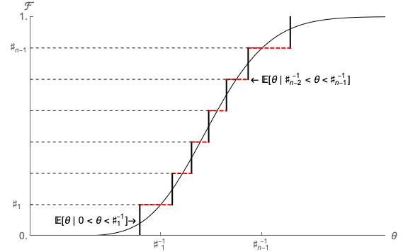

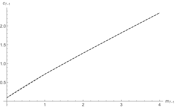
 (solid) versus
  (dashed)
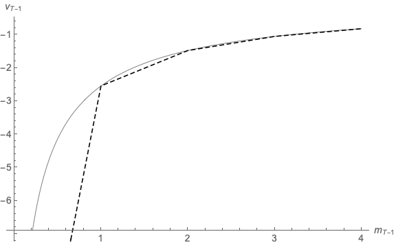
 (solid) versus
  (dashed)
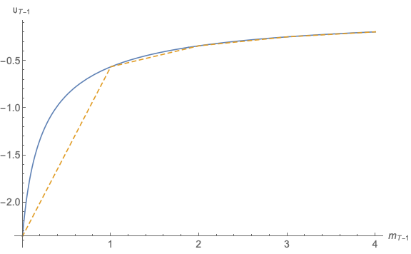
 (solid) versus
  (dashed)
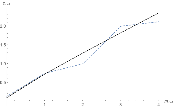
 (solid) versus
  (dashed)
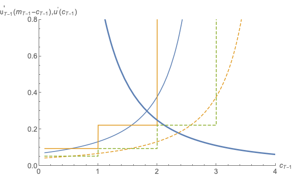
 versus
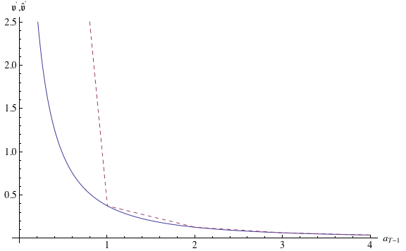
 versus
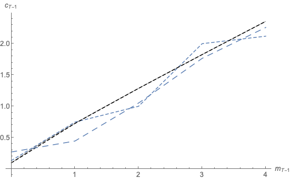
 (solid) Versus Two Methods for Constructing
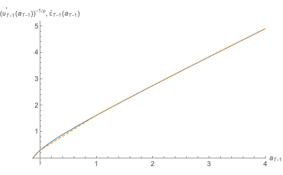
 versus
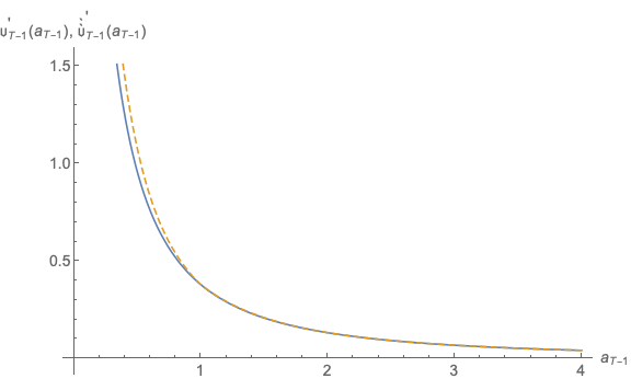
 vs.
vs.  Constructed Using
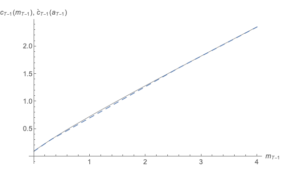
 (solid) versus
  (dashed)
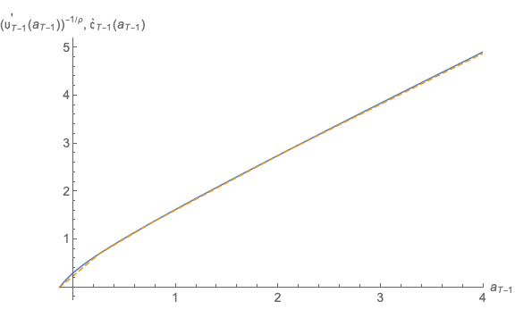
 versus
  , Multi-Exponential
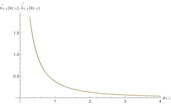
 vs.
vs.  , Multi-Exponential
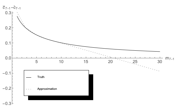
 , Predicted Precautionary Saving is Negative
(Oops!)
, Predicted Precautionary Saving is Negative
(Oops!)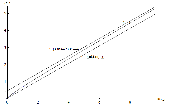

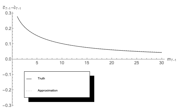
 Constructed Using the Method of Moderation
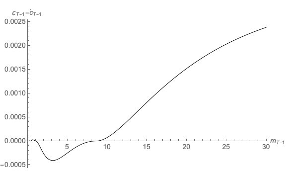
 and
and  Is Minuscule
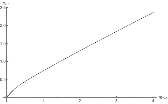
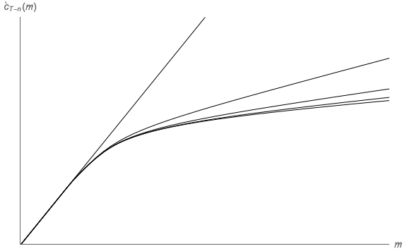
 Functions as
  Increases
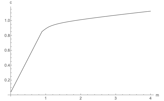
 With Portfolio Choice
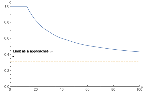

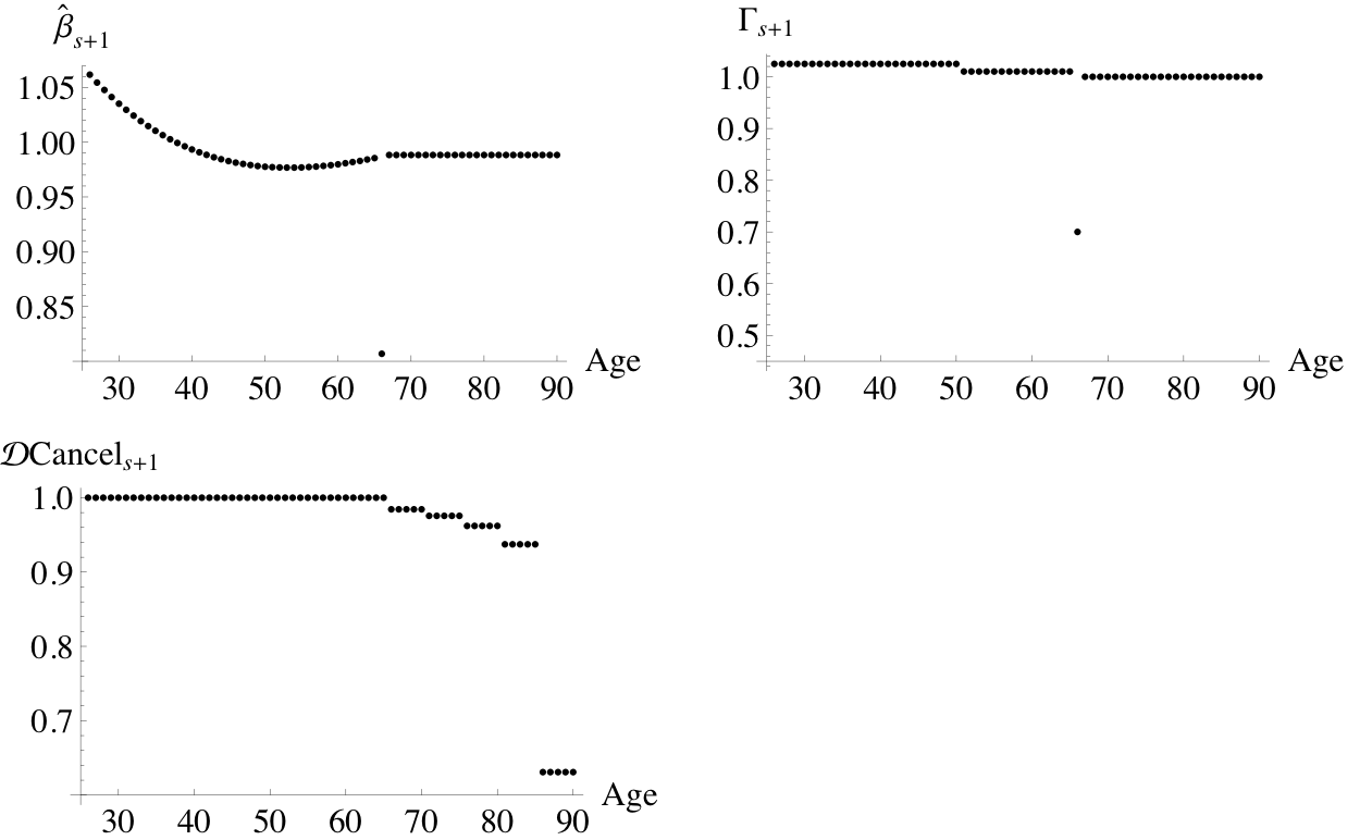

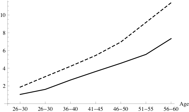

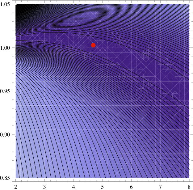
 Estimates (red
dot).
Estimates (red
dot).
 is the predictable (say, life cycle) growth factor
 during the solution stage


