, a transitory shock
  , and the wage rate
  :
:
cstKS, January 24, 2015
_____________________________________________________________________________________
Abstract
A large body of evidence supports Friedman (1957)’s proposition that
household income at the microeconomic level can be reasonably well described as
having both transitory and permanent components. We show how to modify
the widely-used macroeconomic model of Krusell and Smith (1998) to
accommodate a Friedmanesque income process. Our incorporation of
appropriately calibrated permanent income shocks helps our model to explain a
substantial part of the large degree of empirical wealth heterogeneity
that is unexplained in the baseline Krusell and Smith (1998) model.
Household Income Process, Wealth Inequality
D12, D31, D91, E21
| PDF: | http://www.econ2.jhu.edu/people/ccarroll/papers/cstKS.pdf |
| Slides: | http://www.econ2.jhu.edu/people/ccarroll/papers/cstKS-Slides.pdf |
| Web: | http://www.econ2.jhu.edu/people/ccarroll/papers/cstKS/ |
| Archive: | http://www.econ2.jhu.edu/people/ccarroll/papers/cstKS.zip |
1Carroll: Department of Economics, Johns Hopkins University, Baltimore, MD, http://www.econ2.jhu.edu/people/ccarroll/, ccarroll@jhu.edu; and United States Consumer Financial Protection Bureau 2Slacalek: European Central Bank, Frankfurt am Main, Germany, http://www.slacalek.com/, jiri.slacalek@ecb.europa.eu 3Tokuoka: Ministry of Finance, Tokyo, Japan, kiichi.tokuoka@mof.go.jp
The Krusell and Smith (1998) (‘KS’) method for incorporating uninsurable household-level risk into macroeconomic models is a workhorse in macroeconomic modeling. However, the stochastic process that KS use to characterize household income dynamics is strongly inconsistent with microeconomic evidence. Since the point of the KS analysis was to examine quantitative implications of idiosyncratic uncertainty, it is hard to be confident about any of their (quantitative) conclusions if their calibration of the idiosyncratic risk is (quantitatively) implausible.
A large empirical literature, with a history traceable all the way back to Friedman (1957), finds that a simple income process consisting of a permanent and a transitory component—what we call the “Friedman/Buffer Stock” (FBS) process—captures the key features of the microeconomic data well.
In this paper, we solve a modified version of the KS model in which the microeconomic household income process has the FBS structure.
The microeconomic evidence indicates that permanent shocks are large. Consequently, even if households were to start life with the same levels of permanent income, long-lived households will end up differing greatly in their levels of permanent income. Because the model implies the existence of a target ratio of assets to permanent income, the model implies that the equilibrium cross-sectional wealth distribution is roughly as unequal as the distribution of permanent income.
Among the many ways to quantify the importance of our modification, perhaps the most interesting is to note that in our simulations, the top 1 percent of households are almost three times richer than the top 1 percent in the baseline KS model (although even our model falls short of the degree of inequality found in the data).
Friedman (1957) famously characterized income as having permanent and transitory components. A large subsequent empirical literature has confirmed the essential accuracy of this description (see e.g., Meghir and Pistaferri (2011) for a survey of the (vast) literature).2
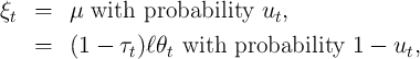
Motivated by Friedman (1957) our household income process consists of
permanent income , a transitory shock , and the wage rate :
Following the assumptions in the the special volume of the Journal of
Economic Dynamics and Control (2010) devoted to comparing solution methods
for the KS model, the distribution of  is:
is:
 is the unemployment insurance payment when unemployed,
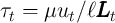 is the rate of tax collected to pay unemployment benefits, and
  is time worked per employee.
Households maximize discounted utility from consumption
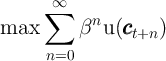 |
for a CRRA utility function 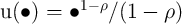 . The aggregate production
function is
. The aggregate production
function is
 | (3) |
where  is aggregate productivity,
  is capital, and
  is aggregate
employment..
is aggregate
employment..
The decision problem for the household in period  can be written using
variables normalized with the level of permanent income
can be written using
variables normalized with the level of permanent income  (e.g.,
 . The consumption functions
  produce levels of
  that
satisfy:
that
satisfy:
 denotes the probability of not dying between periods (see
below),
denotes the probability of not dying between periods (see
below),  is the depreciation factor for capital, and the gross interest rate
  is calculated as marginal aggregate output from capital.
The transition process for market resources  is broken up, for clarity of
analysis, into three steps (5)–(7). Equation (5) indicates that assets at the end of
the period are equal to market resources minus consumption, while next period’s
capital is determined from this period’s assets via equation (6). The final step (7)
describes the transition from the beginning of period
is broken up, for clarity of
analysis, into three steps (5)–(7). Equation (5) indicates that assets at the end of
the period are equal to market resources minus consumption, while next period’s
capital is determined from this period’s assets via equation (6). The final step (7)
describes the transition from the beginning of period  when capital
has not yet been used to produce output, to the middle of that period,
when output has been produced and incorporated into resources but has
not yet been consumed. These steps can of course be combined into
a single transition equation, as is usual in solving problems like this:
when capital
has not yet been used to produce output, to the middle of that period,
when output has been produced and incorporated into resources but has
not yet been consumed. These steps can of course be combined into
a single transition equation, as is usual in solving problems like this:

If the probability of death is  , the FBS income process implies there is
no ergodic distribution of permanent income in the population: Since each
household accumulates a permanent shock in every period, the cross-sectional
distribution of idiosyncratic permanent income becomes wider and wider
indefinitely as the simulation progresses.
, the FBS income process implies there is
no ergodic distribution of permanent income in the population: Since each
household accumulates a permanent shock in every period, the cross-sectional
distribution of idiosyncratic permanent income becomes wider and wider
indefinitely as the simulation progresses.
We address this problem by assuming that households have finite lifetimes a la
Blanchard (1985). Death follows a Poisson process, so that every agent alive at
date  has an equal probability
  of dying before the beginning of period
 . Households engage in a Blanchardian mutual insurance scheme:
Survivors share the estates of those who die. Assuming a zero profit
condition for the insurance industry, the insurance scheme’s ultimate effect
is simply to boost the rate of return (for survivors) by the mortality
rate.
. Households engage in a Blanchardian mutual insurance scheme:
Survivors share the estates of those who die. Assuming a zero profit
condition for the insurance industry, the insurance scheme’s ultimate effect
is simply to boost the rate of return (for survivors) by the mortality
rate.
To maintain a constant population, dying households are replaced by an equal
number of newborns who begin life with idiosyncratic permanent income equal
to the population mean. Mean idiosyncratic permanent income will thus
remain fixed at 1 forever, while the variance of  is finite as long as
![2
//D E[ψ ] < 1](cstKS33x.png) (a requirement that does not do violence to the data).
Intuitively, permanent income among survivors does not spread out so
quickly as to overwhelm the compression of distribution due to death and
replacement.
(a requirement that does not do violence to the data).
Intuitively, permanent income among survivors does not spread out so
quickly as to overwhelm the compression of distribution due to death and
replacement.
We first calibrate the income process using the empirical literature
(see Carroll, Slacalek, and Tokuoka (2014), Table 1, Meghir and
Pistaferri (2011) and many others) and households’ subjective estimates of their
permanent income. In line with this evidence, we set the variance of
the transitory and permanent income components at  and
and  , specifically following the estimates of
Carroll (1992).3
In a sharp contrast, the income process used in the KS model implies estimates
of
, specifically following the estimates of
Carroll (1992).3
In a sharp contrast, the income process used in the KS model implies estimates
of  and
and  that are orders of magnitude different from what the literature
finds in actual data.
that are orders of magnitude different from what the literature
finds in actual data.
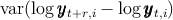
Figure 1 illustrates further the difficulties of the KS process. A key feature
of the data is that the cross-sectional variance of the income profiles
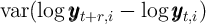 tends to grow linearly with the horizon
  ,
with slope
,
with slope  , mirroring closely the characteristics of the FBS process,
where
, mirroring closely the characteristics of the FBS process,
where  . In contrast, the statistic
for the KS process does not exhibit any trend, also reflecting the fact
that the first autocorrelation of the KS income process is only roughly
0.2.
. In contrast, the statistic
for the KS process does not exhibit any trend, also reflecting the fact
that the first autocorrelation of the KS income process is only roughly
0.2.
As a second check, we make sure that the parameters of the income process are
in line with households’ subjective estimates of their permanent income. The
Survey of Consumer Finances (SCF) conveniently includes a question asking
respondents whether their income in the survey year was about ‘normal’ for
them, and if not, it asks the level of ‘normal’ income. The question corresponds
well with our (and Friedman (1957)’s) definition of permanent income  . We
calculate the cross-sectional variance
. We
calculate the cross-sectional variance  of
of  and, eventually, the
implied variance of
and, eventually, the
implied variance of  . Reassuringly, the estimates of
  from the
1992–2010 SCF data range between 0.015 and 0.018, closely in line with the
estimates reported in Meghir and Pistaferri (2011). Such a correspondence,
across two quite different methods of measurement, suggests there is
considerable robustness to the measurement of the size of permanent
shocks.
from the
1992–2010 SCF data range between 0.015 and 0.018, closely in line with the
estimates reported in Meghir and Pistaferri (2011). Such a correspondence,
across two quite different methods of measurement, suggests there is
considerable robustness to the measurement of the size of permanent
shocks.
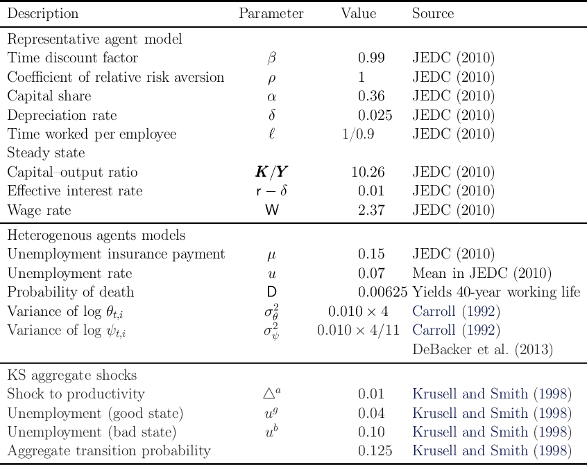
To calibrate the time preference factor  we shut down aggregate uncertainty
and search for the value at which the steady-state capital-to-output ratio
we shut down aggregate uncertainty
and search for the value at which the steady-state capital-to-output ratio  matches the steady-state ratio in the perfect foresight model. Our remaining
parameters match the values in the special JEDC (2010) volume; see Table 2 in
the Appendix.
matches the steady-state ratio in the perfect foresight model. Our remaining
parameters match the values in the special JEDC (2010) volume; see Table 2 in
the Appendix.
We now ask whether our model with realistically calibrated income and finite lifetimes can reproduce the degree of wealth inequality evident in the micro data. An improvement in the model’s ability to match the data (over the KS model) is to be expected, since (as noted above), in buffer stock models agents strive to achieve a target ratio of wealth to permanent income. By assuming no dispersion in the level of permanent income across households, KS’s income process disables a potentially vital explanation for variation in the level of target wealth (and, therefore, on average, actual wealth) across households.
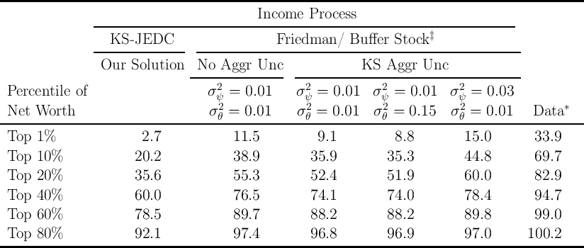
Table 1 shows that the models with the FBS income process (in columns 3 through 6) do indeed yield a substantial improvement in matching the data (in the last column) over the distribution of wealth implied by our solution of the KS model (column 2), as parametrized in the JEDC (2010) volume (which we call ‘KS-JEDC’). For example, in our model with FBS income dynamics and no aggregate uncertainty (column 3), the proportion of total net worth held by the top 1 percent is 11.5 percent, while the corresponding statistic in the KS-JEDC model is only 2.7 percent.
The failure of the KS-JEDC model to match the wealth distribution is not confined to the top. In fact, perhaps a bigger problem is that most households in the model hold wealth levels not very far from the wealth target of a representative agent in the perfect foresight version of the model. For example, in steady state about 50 percent of households have wealth between 0.5 and 1.5 times the mean wealth; in the SCF data from 1992–2004, the corresponding proportion ranges from only 20 to 25 percent.
But while our model fits the data better than the KS-JEDC model, it still falls short of matching the empirical degree of wealth inequality. The proportion of wealth held by households in the top 1 percent is about three times smaller in the model than in the data (compare the third and last columns). This failure reflects the fact that, empirically, the distribution of wealth is considerably more unequal than the distribution of permanent income.4
A comparison of columns 3 and 4 shows that the FBS models without and with KS aggregate uncertainty do roughly equally well in matching the wealth distribution.5 The fact that the specification of aggregate shock has little effect on the performance of the model in this respect is not surprising because it is well-known that aggregate shocks are much smaller than idiosyncratic shocks.
Columns 5 and 6 explore the effects of higher variances of income shocks. A
significantly higher size of transitory shocks (setting  , in line with the
upper range of empirical estimates, DeBacker, Heim, Panousi, Ramnath, and
Vidangos (2013)) results in a stronger precautionary motive and a somewhat
more even wealth distribution. In contrast, allowing for larger permanent shocks
(
, in line with the
upper range of empirical estimates, DeBacker, Heim, Panousi, Ramnath, and
Vidangos (2013)) results in a stronger precautionary motive and a somewhat
more even wealth distribution. In contrast, allowing for larger permanent shocks
( ) implies a less equal wealth distribution (because our model is
scalable with permanent income).
) implies a less equal wealth distribution (because our model is
scalable with permanent income).
Finally, statistics on aggregate dynamics (reported in Carroll, Slacalek, and Tokuoka (2014)) are generally similar for the KS and the FBS models, implying a positive autocorrelation of consumption growth and a high contemporaneous correlation of consumption growth with income growth and interest rates.
This paper has two main results.
First, we have shown how to incorporate a (quantitatively) realistic microeconomic income process in a KS-type model.
Second, we have shown that while this modification substantially improves the fit between the model and the data, the empirically observed degree of inequality is even greater than that implied even by our modified model.
Thus, some mechanism other than shocks to permanent income seems necessary to bring this class of models into full alignment with the available data on wealth inequality (or, another class of models is needed).
BLANCHARD, OLIVIER J. (1985): “Debt, Deficits, and Finite Horizons,” Journal of Political Economy, 93(2), 223–247.
CARROLL, CHRISTOPHER D. (1992): “The Buffer-Stock Theory of Saving: Some Macroeconomic Evidence,” Brookings Papers on Economic Activity, 1992(2), 61–156, http://www.econ2.jhu.edu/people/ccarroll/BufferStockBPEA.pdf.
CARROLL, CHRISTOPHER D., JIRI SLACALEK, AND KIICHI TOKUOKA (2013): “The Distribution of Wealth and the Marginal Propensity to Consume,” mimeo, Johns Hopkins University, At http://www.econ2.jhu.edu/people/ccarroll/papers/cstMPC/.
__________ (2014): “Buffer-Stock Saving in a Krusell–Smith World,” working paper 1633, European Central Bank.
DEBACKER, JASON, BRADLEY HEIM, VASIA PANOUSI, SHANTHI RAMNATH, AND IVAN VIDANGOS (2013): “Rising Inequality: Transitory or Permanent? New Evidence from a Panel of US Tax Returns,” mimeo.
FRIEDMAN, MILTON A. (1957): A Theory of the Consumption Function. Princeton University Press.
JOURNAL OF ECONOMIC DYNAMICS AND CONTROL (2010): “Computational Suite of Models with Heterogeneous Agents: Incomplete Markets and Aggregate Uncertainty,” edited by Wouter J. Den Haan, Kenneth L. Judd, Michel Juillard, 34(1), 1–100.
KRUSELL, PER, AND ANTHONY A. SMITH (1998): “Income and Wealth Heterogeneity in the Macroeconomy,” Journal of Political Economy, 106(5), 867–896.
MEGHIR, COSTAS, AND LUIGI PISTAFERRI (2011): “Earnings, Consumption and Life Cycle Choices,” in Handbook of Labor Economics, ed. by O. Ashenfelter, and D. Card, vol. 4, chap. 9, pp. 773–854. Elsevier.
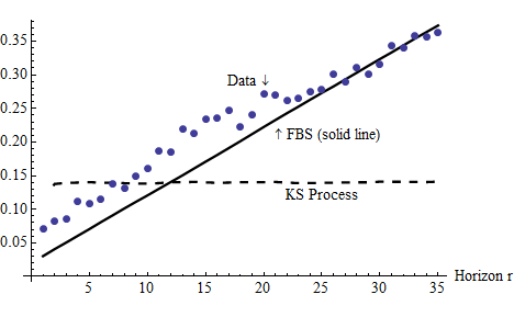
Notes: The data are based on DeBacker, Heim, Panousi, Ramnath, and Vidangos (2013), Figure IV(a) and
were normalized so that the variance for  ,
,  lie in the middle between the values
for the KS and the FBS processes.
lie in the middle between the values
for the KS and the FBS processes.
Notes: 

 when
when  ,
,  when
when
 and
and  when
when  .
.  The data is the SCF
2004.
The data is the SCF
2004.


![[ ]
v(m ) = max u (c ) + β//D E ψ1- ρv(m ) (4)
t ct t t t+1 t+1
s.t.
at = mt - ct, (5)
kt+1 = at∕(//D ψt+1 ), (6)
( )
mt+1 = ℸ + rt+1 kt+1 + ξt+1, (7)
a ≥ 0,
t](cstKS21x.png)