and market wealth
  , spending is given
by
, spending is given
by
Final Version
How Large Are Housing and Financial Wealth Effects? A New Approach
July 4, 2010
| Christopher D. Carroll1 |
| JHU |
| Misuzu Otsuka2 |
| OECD |
| Jiri Slacalek3 |
| ECB |
_____________________________________________________________________________________
Abstract
This paper presents a simple new method for measuring ‘wealth effects’ on
aggregate consumption. The method exploits the stickiness of consumption
growth (sometimes interpreted as reflecting consumption ‘habits’) to distinguish
between immediate and eventual wealth effects. In U.S. data, we estimate that
the immediate (next-quarter) marginal propensity to consume from a $1 change
in housing wealth is about 2 cents, with a final eventual effect around 9 cents,
substantially larger than the effect of shocks to financial wealth. We argue that
our method is preferable to cointegration-based approaches, because neither
theory nor evidence supports faith in the existence of a stable cointegrating
vector.
Housing Wealth, Wealth Effect, Consumption Dynamics, Asset Prices
E21, E32, C22
| PDF: | http://www.econ2.jhu.edu/people/ccarroll/papers/cosWealthEffects.pdf |
| Web: | http://www.econ2.jhu.edu/people/ccarroll/papers/cosWealthEffects/ |
| Archive: | http://www.econ2.jhu.edu/people/ccarroll/papers/cosWealthEffects.zip |
| (Contains data and estimation software producing paper’s results) |
1Carroll: Department of Economics, Johns Hopkins University, Baltimore, MD, http://www.econ2.jhu.edu/people/ccarroll/, ccarroll@jhu.edu 2Otsuka: Organisation for Economic Co-operation and Development, Paris, France, misuzu.otsuka@oecd.org 3Slacalek: European Central Bank, Frankfurt am Main, Germany, http://www.slacalek.com/, jiri.slacalek@ecb.europa.eu.
Conventional wisdom says that the response of household spending to a shock to wealth (the ‘wealth effect’) has historically been around 3 to 5 cents on the dollar in the U.S.2 However, much of the evidence for this proposition comes from ‘cointegrating’ models that regress the level of consumption on the levels of wealth and income.3 ,4
We argue that cointegration methods are problematic for estimating wealth effects, for at least two reasons.5 First, basic consumption theory does not imply the existence of a stable cointegrating vector; in particular, a change in the long-run growth rate or the long-run interest rate should change the relationship between consumption, income, and wealth.6 Second, even if changes to the cointegrating vector are ruled out by assumption, changes in any other feature of the economy relevant for the consumption/saving decision can generate such long-lasting dynamics that hundreds or thousands of years of data should be required to obtain reliable estimates of that vector.
Even for the U.S., the technological leader and therefore the most stable advanced country in the modern era, the 50 year span of available data has seen major changes in productivity growth, interest tax rates, demographics, financial markets, social insurance, and every other aspect of reality that theory says should matter for consumption (not to mention fundamental changes in measurement methods for the underlying NIPA data).
Motivated by these concerns, we introduce an alternative methodology for estimating wealth effects. The method’s foundation derives from the recent literature documenting substantial ‘excess smoothness’ (or ‘stickiness’) in consumption growth, relative to the benchmark random walk model.7 Our model can be thought of as a proposal for unifying the ‘stickiness’ and the ‘wealth effects’ literatures, by resolving wealth effects into two key aspects: Speed and strength.
Our measure of ‘speed’ is meant to distill and quantify the core point of the stickiness literature: Consumption responds to shocks more slowly than implied by the random-walk benchmark. Given an estimated ‘speed,’ our measure of the ‘strength’ of wealth effects is thus dependent on the horizon; our ‘speed’ estimates imply that the immediate spending effects of wealth fluctuations are much smaller than the eventual effects.8 In particular, we find that the immediate (next-quarter) marginal propensity to consume (MPC) from a $1 change in housing wealth is about 2 cents, with an eventual effect amounting to 9 cents. Consistent with several other recent studies, we find a housing wealth effect that is larger than the financial wealth effect, which we estimate to be about 6 cents on the dollar.
These differing estimates suggest that markets and policymakers worried about wealth effects may need to pay careful attention not only to the size of overall changes in total wealth but also to how those wealth changes break down between different asset classes.
This section uses a simple model of consumption to illustrate why a cointegrating approach may not correctly identify the wealth effect (even when it exists), and shows how the new method that we propose addresses this shortcoming.
In the benchmark perfect foresight model with no uncertainty, perfect capital
markets, homogenous consumers and no bequest motive, steady-state
consumption is proportional to overall resources. If total resources are the sum of
nonmarket (human) wealth and market wealth , spending is given
by
 | (1) |
where κ is a constant determined by preferences and the
after-tax interest factor R = 1 + r (assumed here to be
constant).9
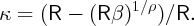
In the version of the model with infinitely lived consumers, constant relative risk
aversion ρ, and the discount factor β =  the MPC takes the explicit
form
the MPC takes the explicit
form
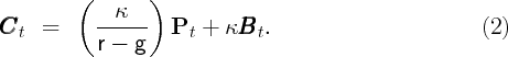
If labor income is expected to grow at a constant rate g, then (in the
continuous-time approximation)  t will be given by Pt∕(r -g) where
Pt is the current value of ‘permanent’ labor income, and (1) becomes
t will be given by Pt∕(r -g) where
Pt is the current value of ‘permanent’ labor income, and (1) becomes
This model can be extended to the case with i.i.d. interest rates
(cf. Merton (1969) and Samuelson (1969)), which adds a term to the formula
for κ but does not change the structure of (2). In this case the stochastic interest
rate would result in ‘wealth shocks’ to  t.
t.
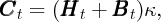
The cointegrating approach to estimating the model would be to assume that consumption is determined by an equation like (2) plus an error perhaps reflecting transitory shocks to consumption or measurement problems, leading to a regression of the form

 t proxies for Pt and with the hope
that the coefficient η2 will uncover the MPC out of wealth, κ. (This is, of course,
a simplification of actual practice, but it captures the essence of the
method.)
t proxies for Pt and with the hope
that the coefficient η2 will uncover the MPC out of wealth, κ. (This is, of course,
a simplification of actual practice, but it captures the essence of the
method.)
Unfortunately, almost any attempt to make the model more realistic destroys
the prediction that there is a time-invariant ‘wealth effect’ coefficient κ. In the
simple model sketched above, it is clear that any sustained change in g, r, ρ, or ϑ
during the estimation interval would pose serious problems because no
time-invariant κ exists even under the usual maintained assumption that
movements in  t represent exogenous shocks; this point holds with even
greater force if those ‘wealth shocks’ to
t represent exogenous shocks; this point holds with even
greater force if those ‘wealth shocks’ to  are correlated with persistent
movements in g, r, ρ, or ϑ (as asset pricing theory suggests they will
be).10
are correlated with persistent
movements in g, r, ρ, or ϑ (as asset pricing theory suggests they will
be).10
Even if we assume perpetual constancy in g, r, ρ, and ϑ, the model’s prediction of a time-invariant κ can be destroyed by the introduction of labor income uncertainty, time-varying after-tax interest rates, demographics, or many other real-world complications.
Such concerns are given further force by the large econometric literature on ‘spurious significance’ that can result from regressing non-stationary variables on each other, the upshot of which is that econometric tests may appear to detect a significant relationship even when the variables are actually independent.
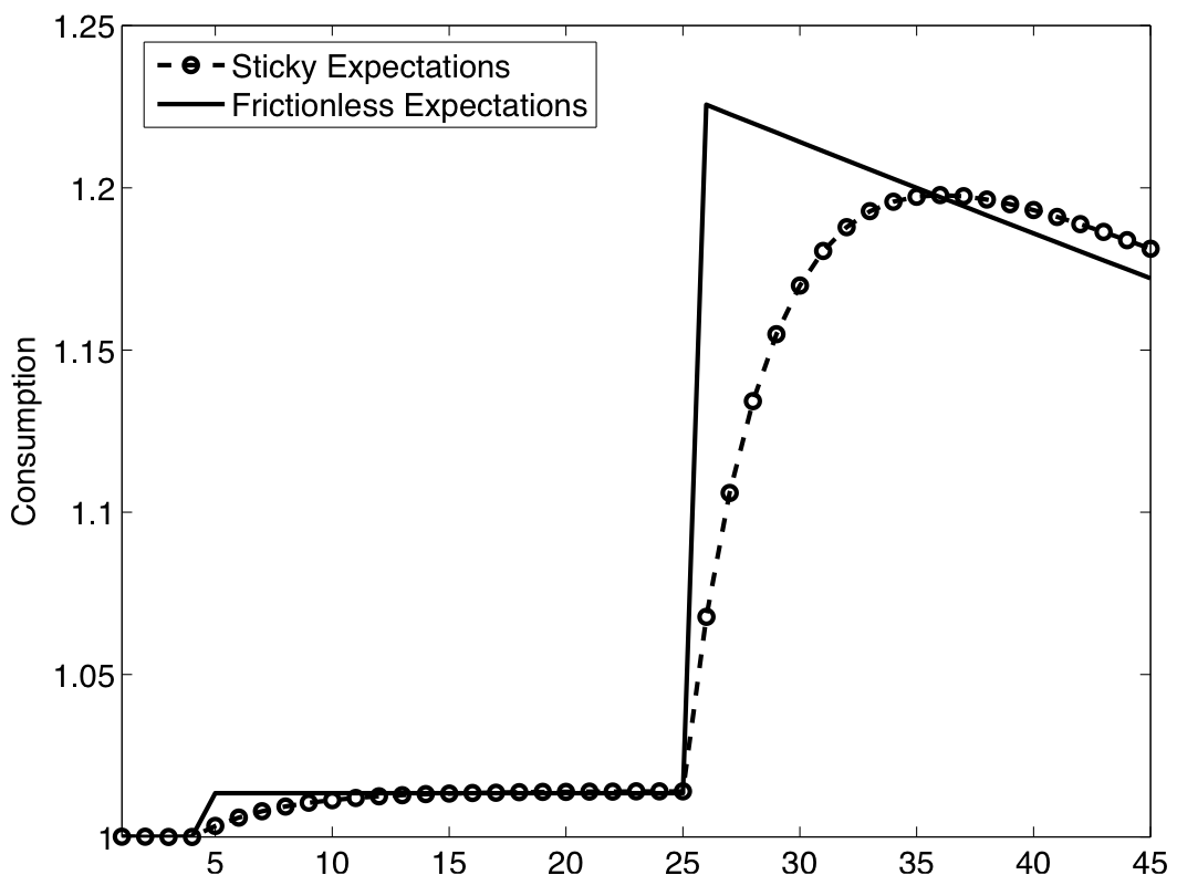
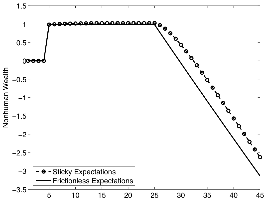
As a specific illustration of the problem we are concerned about, consider the following scenario, illustrated in figures 1(a) and 1(b). (Plain solid lines show the reactions of consumption and wealth (normalized by income; hence nonbold) for the ‘frictionless’ model sketched above.) The economy starts in period 1 in a steady state balanced growth equilibrium in which B = 0 and C = 1, and stays in that equilibrium for 4 periods. In period 5 it is hit with a 1-unit positive shock to wealth so that B5 = 1. The economy evolves with no further shocks for n = 20 quarters, then in period 25 experiences a permanent increase in income growth g.11 The simulation runs for another 20 periods, ending in period 45.12
Consumption adjusts upward immediately (in period 5) to the period-5 wealth shock; both consumption and wealth remain constant thereafter. Thus, the size of the ‘wealth effect’ κ on consumption can be measured directly by comparing the change in consumption to the change in wealth. This is the ‘best-case scenario’ for measuring a wealth effect.
The expected growth rate of income g is the object that we modify in order to produce our experiment’s second shock. When this positive growth shock hits, consumption jumps up to a much higher level; but nonhuman wealth B begins to fall, because, now, spending exceeds income. This dissaving reflects the ‘human wealth’ effect emphasized by Summers (1981): When consumers become more optimistic about future income growth, they start spending today on the basis of their anticipated future riches. But as consumption continues to exceed current income, the ratio of nonhuman wealth to income B declines, and the ratio of consumption to income C also declines. Both C and B thus embark on downward trajectories after the shock; but B falls starting from its pre-shock level, while C starts falling only after having made a one-time upward leap because of the human wealth effect.
This experiment provides a clear example in which, even though a ‘marginal propensity to consume out of wealth’ unambiguously exists (κ ≈ 0.014) in the underlying structural model, it cannot be uncovered by estimating a supposed ‘cointegrating’ regression of consumption on wealth. Indeed, the coefficient obtained from such a regression would actually be negative, because after the positive income-growth shock, consumption is higher on average than before the shock, while average wealth after the shock is lower than before the shock.
Table 1 presents the quantitative results for the (n = 20) experiment illustrated in the figures, as well as for similar experiments with 40 and 60 quarters.13 As long as the shocks occur more frequently than about every 15 years (= 60 quarters), regressions of consumption C on wealth B estimate a negative wealth effect, even though the true parameter of interest is about 0.014. While cointegrating regressions eventually do provide consistent estimates as n approaches infinity and if there are no more shocks, Table 1 suggests that convergence of the cointegrating estimates to the truth is likely to be too slow to make cointegration estimation a reliable method of uncovering structural parameters (even if they exist) over the (relatively) short spans of time captured in actual empirical macroeconomic datasets.
This section argues that if there is a reliable degree of ‘stickiness’ in consumption growth, an estimation method that relies upon that stickiness to estimate wealth effects using high- and medium-frequency data is less likely to be led astray by a ‘regime change’ (like the one examined above) than a full-sample estimation technique like cointegration estimation.
Consumption habits are the leading explanation for sluggishness in aggregate
consumption. But an alternative explanation is that households may be
mildly inattentive to macroeconomic developments—for example, some
households may not immediately notice shocks to aggregate macroeconomic
indicators such as productivity growth or the unemployment rate. Carroll and
Slacalek (2006) simulate an economy consisting of a continuum of such
inattentive but otherwise-standard consumers with Constant Relative
Risk Aversion utility, each of whom updates the information about his
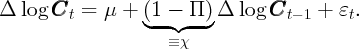
permanent income with probability Π in each period. They show that the
change in the log of aggregate consumption, Δ log  t, approximately
follows an autoregressive AR(1) process, whose autocorrelation coefficient
approximates the share of consumers (1 - Π) who do not have up-to-date
information:
t, approximately
follows an autoregressive AR(1) process, whose autocorrelation coefficient
approximates the share of consumers (1 - Π) who do not have up-to-date
information:
 | (3) |
Exactly the same approximation can be obtained for some models of habit-forming consumers, e.g., Muellbauer (1988) and Dynan (2000), but the coefficient χ in those models measures the intensity of the habit motive. When we estimate a model of the form of equation (3), our estimates cannot distinguish between these alternative hypotheses about the reason for stickiness.14 But, from the standpoint of forecasting aggregate consumption dynamics, it may not matter whether the right explanation of stickiness is habits or inattention.
As an illustration of how our estimation method works, consider the behavior of aggregate consumption and wealth in the same economy described in the previous section, except that consumption is now that of inattentive households who update their information on average once a year (i.e., Π = 0.25 or χ = 0.75). The dashed lines in Figures 1(a) and 1(b) show the gradual adjustment of the two variables, which occurs because some consumers remain unaware of the shocks for several quarters. This sluggishness provides an informative signal to identify parameters of interest.
Table 2 uses an equation like the one we will estimate empirically below,

 t-1 rather than Δ
 t as the second regressor.)
The regression captures the essence of our estimation approach, whose empirical
implementation is detailed in section 3. The two key findings in the table are: (i)
the stickiness parameter χ lies close to its true value, and (ii) the estimates of
the wealth effect are broadly in line with the ‘true’ value calculated from the
calibrated parameters, 0.014. As for the latter, the estimated wealth effect
decreases somewhat for n = 60, which suggests that enough shocks are needed to
identify the parameters; but, shocks presumably arrive in the real world
more often than once every 60 periods (15 years), so this finding is not
especially troubling for our hopes of estimating the model with empirical
data.
t as the second regressor.)
The regression captures the essence of our estimation approach, whose empirical
implementation is detailed in section 3. The two key findings in the table are: (i)
the stickiness parameter χ lies close to its true value, and (ii) the estimates of
the wealth effect are broadly in line with the ‘true’ value calculated from the
calibrated parameters, 0.014. As for the latter, the estimated wealth effect
decreases somewhat for n = 60, which suggests that enough shocks are needed to
identify the parameters; but, shocks presumably arrive in the real world
more often than once every 60 periods (15 years), so this finding is not
especially troubling for our hopes of estimating the model with empirical
data.
We should emphasize here that the foregoing is presented more in the spirit of illustration of our ideas than as a rigorous treatment of a theoretical model. We think of our method as a first stab at the problem of providing a robust but cointegration-free method for estimating dynamic wealth effects, and we hope that more rigorous modeling and structural estimation will follow. But we anticipate that such approaches will confirm the basic dynamics captured by our method, in part because we think those dynamics have been reflected in the results obtained in most of the recent literature on structural estimation of more complicated macroeconomic models, which invariably find a strong component of ‘habit formation.’
Our method also has the advantage that it allows for a transparent
generalization for comparing the effects of shocks to different kinds of wealth. If
housing wealth is measured by  th and financial wealth by
  tf, our method
boils down to estimating
tf, our method
boils down to estimating

Our estimation approach exploits the robust empirical fact that aggregate consumption growth responds only sluggishly to shocks. The most persuasive evidence that such sluggishness exists is the reluctant introduction of habits into quantitative macroeconomic models in the last few years, despite the evident distaste for the habit formation assumption on the part of many researchers. Models that include habits are proliferating because they can match the core empirical fact of sluggish consumption growth along with attendant implications for asset pricing and other empirical phenomena.
In implementing our method in actual data, the first step is to estimate the degree of stickiness in consumption growth in (3). But there is a problem: The producer of the consumption data documents a variety of sources of measurement error in that data (Bureau of Economic Analysis, 2006). Furthermore, anyone who has been involved in real-time consumption forecasting knows that there are large transitory elements of spending (e.g. hurricane-related purchases) that are not incorporated in the theory that leads to (3).
Fortunately, these problems can be largely overcome when χ is estimated with instrumental variables estimation using instruments dated t - 2 or earlier.17 These estimates suggest a serial correlation coefficient for ‘true’ consumption growth in the neighborhood of 0.7 (whether the measure of spending is total consumption expenditures, spending on nondurables and services, or spending on nondurables alone). The evidence below confirms that this finding holds robustly for alternative sets and alternative lags of instrumental variables.
To estimate the wealth effect, we must modify Sommer’s methodology in several directions. First, the ultimate goal here is to obtain an estimate of the marginal propensity to consume out of wealth. But (3) is written in terms of the growth rate of consumption. Even if the model were estimated as a just-identified system where the only instrument for lagged consumption growth is lagged changes in wealth, the result would be a relationship between the growth rate of wealth and the growth rate of consumption, which is not an MPC. Worse, this approach makes no sense if wealth is split up into a housing and a financial component. If the null hypothesis is that the MPCs out of the two components are equal then the coefficients on their log changes will not be identical unless financial and housing wealth are the same size in every period (in which case their differential effects would not be identified!).
There is a simple solution to these problems, which is to use the ratio of changes in wealth to an initial level of consumption rather than wealth growth.18 That is, if we define
and so on, then a first-stage regression of the form yields a direct estimate of the marginal propensity to consume in quarter t out of a change in wealth in quarter t- 1. Furthermore, if f and
f and  h are the financial
and housing components of wealth, a first-stage regression of the form
yields directly comparable estimates of relative MPCs.
h are the financial
and housing components of wealth, a first-stage regression of the form
yields directly comparable estimates of relative MPCs.
The reader may wonder why the wealth variables in (5) are lagged one period. This is for several reasons. First, wealth in our source (the Flow of Funds Accounts) is measured at a point in time (on the last day of the quarter), while consumption occurs continuously throughout a quarter. If we were to use a measure of wealth with the same time subscript as our measure of consumption, in practice that would be incorporating information that was revealed to the consumer only late in the quarter as though the consumer could have known about it early in the quarter. Second, there is a potentially serious simultaneity problem with looking at the relationship between current consumption and current wealth: Maybe innovations to both are driven by some exogenous unmeasured third variable (growth expectations, say). Then if asset markets respond instantly to new information (as they should to prevent arbitrage; the random walk proposition is much closer to holding true for asset prices than for consumption), the coefficient on wealth would reflect some of this simultaneity bias rather than a ‘pure’ marginal propensity to consume. Finally, the most useful context in which empirical work like this might be performed is in forecasting high frequency consumption movements. To do that, one needs to have lagged, not contemporaneous, variables on the right hand side.
Regressions of the form (4) or (5) pass all the standard tests of instrument validity and therefore justify estimation of an IV equation of the form
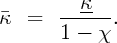
where γ is an unimportant constant. Given an initial (current-quarter) MPC out of wealth of κ and a serial correlation
coefficient χ for ∂ , the usual infinite horizon formula implies that the ultimate effect
on the level of consumption (the ‘eventual MPC’) from a unit innovation to wealth
is19
, the usual infinite horizon formula implies that the ultimate effect
on the level of consumption (the ‘eventual MPC’) from a unit innovation to wealth
is19
Our interpretation of the econometric object we call the ‘eventual MPC’ is that it really reflects the medium-run dynamics of consumption (over the course of a few years); that is, the effects over a time frame short enough that the consequences of the consumption decisions have not had time to have a substantial impact on the level of wealth and to induce general equilibrium offsets. Thus the distinction between what we are calling the ‘eventual’ MPC and what comes out of a cointegration analysis is that in principle the cointegration analysis characterizes some average characteristics of the whole 45-year sample, while our results reflect average dynamics over a much shorter horizon.
Returning to the main thrust, the simplest way to estimate the “eventual
MPC” would have been to directly report the relevant coefficient estimates on
one-quarter-lagged ∂ from the first-stage regressions. If that MPC had been α
then the fact that α = χκ implies that the eventual MPC could have been
estimated from
from the first-stage regressions. If that MPC had been α
then the fact that α = χκ implies that the eventual MPC could have been
estimated from
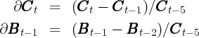
However, the coefficient estimates when only a single lag of each of the two measures of wealth was included in the regression were a bit too sensitive to the inclusion of other instruments for us to be comfortable relying upon them directly.20 However, if the model of serial correlation in true consumption growth is right, it is easy to make an alternative measure of the change in wealth that should capture the relevant facts. For a given value of χ, assuming independent shocks to wealth from quarter to quarter we should have:

Now define
and since similarly ∂ t = (
t = ( t -
t - t-1)∕
t-1)∕ t-5 this leads to an approximate
equation for ∂
t-5 this leads to an approximate
equation for ∂ and
and  of the form Under the assumption that the dynamic model of consumption is right, the
coefficient estimate on
of the form Under the assumption that the dynamic model of consumption is right, the
coefficient estimate on  t should be the immediate (first-quarter) MPC out of
an innovation to wealth.
t should be the immediate (first-quarter) MPC out of
an innovation to wealth.
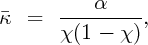
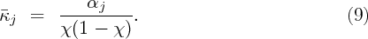
Thus, the estimate of the eventual MPC out of wealth reported in table 4 is given by
for the αj, j ∈{f,h} corresponding to the respective measure of wealth.To summarize, for each of the instrument sets, the procedure is as follows:
 as per (7).
The logic of the foregoing is admittedly a bit circular, but the circularity is motivated more by presentational issues than substance: It seemed essential, for streamlined exposition, to be able to report a single statistic as the immediate MPC and a single statistic as the eventual MPC out of wealth shocks. However, when only a single lag of wealth is used in the first-stage regression the coefficient estimates are implausibly sensitive to the exact specification and exactly which instruments are included. When a few lags are used, the sum of the coefficients on the lags tends to yield similar immediate coefficients, but is harder to summarize. Hence the compromise represented by table 3.
As a baseline, the first row of table 3 presents the estimation results of the
regression (8) of the change in consumption ∂ t on a weighted average of the
change in wealth over the prior year
t on a weighted average of the
change in wealth over the prior year  t-1. Thus, the regression coefficients are
now interpretable as the marginal propensity to consume out of changes in
wealth in the previous quarter. The reported results are for total personal
consumption expenditures (PCE), because the focus here is on the effects of
wealth on aggregate demand, but appropriately scaled-down results can be
obtained for spending excluding durables, or excluding both durables and
services.
t-1. Thus, the regression coefficients are
now interpretable as the marginal propensity to consume out of changes in
wealth in the previous quarter. The reported results are for total personal
consumption expenditures (PCE), because the focus here is on the effects of
wealth on aggregate demand, but appropriately scaled-down results can be
obtained for spending excluding durables, or excluding both durables and
services.
The coefficient estimate in this baseline model implies that if wealth grew by
$1 last quarter, then consumption will grow by about $0.017 more in the current
quarter than if wealth had been flat. While this wealth effect is highly
statistically robust, lagged wealth growth alone explains only about 14
percent of quarterly consumption growth (as implied by the 2 from the
regression of ∂ t on a constant and
  t-1,…,
 t-4 not reported in table
3).21
t-4 not reported in table
3).21
The next step is to find a parsimonious set of additional variables that have significant predictive power for consumption growth. There is a traditional set of variables often used in this literature, dating back to the work of Campbell and Mankiw (1989), including the recent performance of stock prices as well as lagged interest rates and income growth rates. However, for our purposes an adequate representation is obtained by augmenting lagged wealth with just two explanatory variables: Lagged unemployment expectations from the University of Michigan’s consumer sentiment survey (to capture changes in economic uncertainty), and the lagged Fed funds rate, which is included in the hope that it will capture some of the effects of monetary policy, leaving the housing wealth variable to capture more exogenous movements in house prices.
The second row shows that when the extra variables are added, the coefficient on the change in wealth is diminished (by about half). This makes sense because the extra variables are correlated with the change in wealth. However, the extra variables also have considerable independent predictive power for consumption growth. Overall, the explanatory power of the regression including both extra measures is almost double the power of the regression that only includes lagged wealth.
The third row regresses the consumption change on the change in housing and financial wealth separately; the point estimate of the effect of housing wealth is more than twice as large as the coefficient on financial wealth (which is close to the original estimate of the effect of total wealth). However, the coefficient on housing wealth is much less precisely estimated than the coefficient on financial wealth, and a statistical test indicates that the hypothesis that the two coefficients are actually equal cannot be rejected at the 95 percent significance level. One reason the coefficient on housing wealth is harder to pin down is that housing wealth varies considerably less than financial wealth, as shown in figure 2.
The final row presents our preferred specification, in which financial and housing wealth effects are examined separately from the other explanatory variables. Results are broadly what would be expected from the foregoing: Both coefficients are substantially smaller, and the coefficient on housing wealth is about twice as large as that on financial wealth, but the difference between the two coefficients is not statistically significant. The coefficient on housing wealth is different from zero, at the 0.14 percent level.
The results in this table are not the bottom line, because they reflect only the next-quarter effect on consumption growth. To obtain the eventual MPCs, we need to estimate equation (6) and apply formula (9). Results of these calculations are reported in table 4.
The first column shows that all models find a very substantial, and highly
statistically significant, amount of momentum (by which we mean an estimate
of χ > 0) in consumption growth. Note also that the regressions that
include the extra explanatory variables (which had much greater power
for consumption growth) find notably higher estimates of momentum.
Furthermore, in experiments not reported here (but available in the replication
archive), a much more extensive set of instruments was examined. The
bottom line is that any instrument set that has a reasonable degree of
predictive power for ∂ t (e.g., an 2 of 0.1 or more) generates a highly
statistically significant estimate of the χ coefficient. Furthermore, the estimate
of χ tends to be larger the better is the performance of the first-stage
regression.
t (e.g., an 2 of 0.1 or more) generates a highly
statistically significant estimate of the χ coefficient. Furthermore, the estimate
of χ tends to be larger the better is the performance of the first-stage
regression.
The last two columns report the estimated eventual MPCs out of financial and housing wealth. When the MPCs are permitted to differ for financial and housing wealth, the higher immediate MPCs out of housing wealth from table 3 translate into higher eventual MPCs here, with the preferred model estimate (the last row) of an eventual MPC out of housing wealth of 9 cents on the dollar.
One intuition for why the MPC out of financial wealth is substantially lower than that out of housing wealth is evident in figure 2. Financial wealth is considerably more volatile than housing wealth. If the model is really true, these high frequency fluctuations should have considerable power in explaining subsequent spending patterns. In practice, high frequency stock market fluctuations do not seem to translate into very large subsequent consumption fluctuations, so the coefficient is not estimated to be very large.22
The work most closely related to ours is Case, Quigley, and Shiller (2003) (henceforth CQS), which provides estimates from both a panel of developed countries (since 1975) and a panel of states within the U.S. Using annual data, CQS find a highly statistically significant estimate of the MPC out of housing wealth in the U.S. of around 0.03–0.04. In contrast, the CQS estimate of the MPC out of stock market wealth is small and statistically insignificant. The coefficient on housing wealth is estimated to be highly statistically significantly larger than the coefficient on financial wealth.
But the literature does not speak with one voice. A study by Ludwig and Slok (2004) estimates a larger effect of financial wealth than housing wealth in a panel of 16 OECD countries, and also reports some evidence of an increase in wealth effects over time. Girouard and Blöndal (2001) fail to find consistent results across countries: In some, the housing wealth effect is stronger, while in others the financial wealth effect is stronger (and in some neither was significant). And a study by Dvornak and Kohler (2003) modelled closely on the CQS study but using Australian state-level data finds a larger financial wealth effect than housing wealth effect.
It should be admitted that there are good reasons to be skeptical of results based on macroeconomic or regional data (including our own). Foremost among these is the previously-acknowledged point that movements in asset prices are not exogenous fluctuations; they should be affected by many of the same factors that affect consumption decisions, most notably overall macroeconomic prospects. House prices should depend, in part, on the overall future purchasing power of current and future homeowners, while stock prices should reflect expectations for corporate profits, which are of course closely tied to the broader economy. John Muellbauer and various co-authors (Aron and Muellbauer, 2006, Muellbauer, 2007, Aron, Duca, Muellbauer, Murata, and Murphy, 2008) (using Japanese, South African, U.K. and U.S. data) have attempted to address this problem by including control variables for credit market liberalizations and other time varying conditions. But to isolate a ‘pure’ housing wealth effect, one would want data on spending by individual households before and after some truly exogenous change in their house values, caused for example by the unexpected discovery of neighborhood sources of pollution.
The perfect experiment observed in the perfect microeconomic dataset is not available. Many authors have attempted to measure housing wealth effects using microeconomic datasets, but heroic assumptions usually must be made in order to produce estimates, because the existing datasets were not designed with this question in mind.
Given these problems, it is not surprising that the results from microeconomic studies are even more heterogeneous than those from macroeconomic data.
Recent studies by Attanasio, Blow, Hamilton, and Leicester (2008), and Campbell and Cocco (2006) represent both the wide spectrum of views and the best available microeconomic evidence and methodologies.
Disney, Gathergood, and Henley (2008) find an MPC out of unanticipated shocks to housing wealth of only 0.01, after controlling for expectations of future financial conditions. They show that without such controls, the estimated MPC is considerably higher, a result that strongly suggests that the macroeconomic correlation evident in both U.K. and U.S. data reflects causality from general economic conditions to both consumption and asset prices, rather than a direct housing wealth effect.
On the other hand, Campbell and Cocco (2006) also use British data (this time, from the U.K. Family Expenditure Survey and from regional house price surveys), but find a large housing wealth effect, which is different for young and old households; they find a statistically significant elasticity of consumption to house prices of about 1.7 among older homeowners, but no significant effect among young renters.
Attanasio, Blow, Hamilton, and Leicester (2008), in contrast, find that consumption of young renters is positively associated with house price changes, which again suggests that both consumption and house prices are responding to an unobserved aggregate. Additional microeconometric estimates of the wealth effect are reported in Engelhardt (1996), Juster, Lupton, Smith, and Stafford (2001), Lehnert (2003), Levin (1998) and Bostic, Gabriel, and Painter (2005).
Stepping back from the conflicting details of the disparate studies, perhaps the most useful observation is that even if it is true that the ‘pure’ housing wealth effect is modest, if a macroeconomic policymaker wants to know what to expect for future consumption growth given a particular recent path of aggregate wealth shocks, it may matter more whether the forecast is reliable than whether the mechanism is a direct wealth effect, a reflection of an omitted variable like growth expectations, or a reflection of a difficult-to-measure variable like credit conditions. If, for example, a collapse in house prices properly signals a collapse in consumption, the precise mechanism by which consumption will collapse may not be so important.
Despite the obvious limitations of aggregate data, we now attempt to decompose the total response of spending to wealth into the parts due to the five channels outlined above in section 2:23 1. The ‘statistical’ effect because the stream of housing services is included in total PCE and depends on housing wealth, 2. The possibility that the MPC out of a particular kind of wealth might depend on its degree of liquidity, 3. Collateral constraints might be important; and 4. The cross-sectional distribution of wealth might matter.
To address the relevance of the statistical effect, we have re-estimated the model measuring consumption with total PCE excluding housing services. The results are in line with our baseline: The housing wealth effect (h = 0.070) remains highly statistically significant and roughly twice as large as the financial wealth effect (f = 0.039). As a caveat it is worth mentioning that this alternative specification addresses the problem only when utility is additively separable in housing services and the rest of PCE.24
The second and third channels are difficult to assess separately and are both driven by financial innovation. Iacoviello and Neri (2007) argue that the recent increase in liquidity of housing is captured in the higher loan-to-value (LTV) ratio.25 In addition, as pointed out by Muellbauer (2007), the rise in LTV ratios (and the reduction in down-payments) increases consumption of young credit-constrained first-time home buyers. On the other hand, the falling relevance of credit constraints (both in terms of the number of households they affect and their extent) has likely weakened the wealth effect.26
Muellbauer (2007) constructs an indicator of credit market conditions based on the Federal Reserve’s Senior Loan Officer Survey question about the willingness of banks to make consumer installment loans (see the installment loans credit indicator in Figure 4 of his paper). Possibly because of the deregulation and restructuring of the U.S. housing finance system (see e.g., McCarthy and Peach, 2002), the indicator rose markedly around 1984, a movement which likely drives much of the significant increase in the housing wealth effect reported by Muellbauer (2007). The split-sample regressions (pre-1985 and post-1984) we have estimated with our method confirm this finding: The eventual housing wealth effect rose from only 0.03 to 0.12 (while the financial wealth effect actually fell from 0.08 to 0.03).27 Much of the recent literature thus seems to agree that the impact of housing wealth on consumption has been rising in a period (post-1985 or so) which coincides with the intense financial innovation. This evidence is suggestive of a potential causal link. (Of course, as in many other applications, econometric methods like ours do not make it possible to make a final conclusion on the direction of causality.) Our split-sample regressions thus point to a substantial role of financial innovation (channels number 2 and 3) in determining the size of the housing wealth effect. While there are many distinct ways in which financial markets affect the transmission between wealth and consumption, on balance it does seem likely that financial innovation may have made consumption more responsive to housing wealth shocks.
The fourth channel that might affect the size of the wealth effect on aggregate level
is the cross-sectional distribution of various classes of assets. Estimates with aggregate
data implicitly identify the marginal propensity to consume out of wealth averaged
across households: κ = (1∕N) ∑
i=1Nκi( i)ωi, where the marginal propensity
κi28 of
each consumer decreases with his wealth
i)ωi, where the marginal propensity
κi28 of
each consumer decreases with his wealth  i (due to the diminishing role of the
precautionary saving motive), and ωi is the household’s weight in the aggregate
statistic. Housing is considerably more evenly distributed than financial assets:
In the U.S. Survey of Consumer Finances (SCF) of 2004 the top five percent of
households (by net worth) held 26.3 percent of the total value of houses
(or $5.0 trillion) but 57.9 percent of financial assets (or $12.2 trillion)
(see Kennickell, 2006, Table 11a). Unfortunately, it is difficult to assess
quantitatively by how much the aggregate MPC out of housing wealth would fall
if we exogenously imposed that housing has the same distribution as financial
assets.29
However, it is well-known that both housing and financial wealth of the richest
households has since 1995 grown very rapidly (see, e.g., Survey of Consumer
Finances, 2007).30
This shift has probably, if anything, weakened wealth effects. However, the
change seems likely to be modest because theory suggests that the spending
of the rich people should not react much to shocks (both because of
the weak precautionary saving motive and the irrelevance of liquidity
constraints).
i (due to the diminishing role of the
precautionary saving motive), and ωi is the household’s weight in the aggregate
statistic. Housing is considerably more evenly distributed than financial assets:
In the U.S. Survey of Consumer Finances (SCF) of 2004 the top five percent of
households (by net worth) held 26.3 percent of the total value of houses
(or $5.0 trillion) but 57.9 percent of financial assets (or $12.2 trillion)
(see Kennickell, 2006, Table 11a). Unfortunately, it is difficult to assess
quantitatively by how much the aggregate MPC out of housing wealth would fall
if we exogenously imposed that housing has the same distribution as financial
assets.29
However, it is well-known that both housing and financial wealth of the richest
households has since 1995 grown very rapidly (see, e.g., Survey of Consumer
Finances, 2007).30
This shift has probably, if anything, weakened wealth effects. However, the
change seems likely to be modest because theory suggests that the spending
of the rich people should not react much to shocks (both because of
the weak precautionary saving motive and the irrelevance of liquidity
constraints).
Table 5 demonstrates the robustness of our estimates of the wealth effects to
three alternative specifications of the model. The top panel considers an
alternative instrument set for lagged consumption growth  t-1 in (6), which
consists of the growth rate of stock prices, change in unemployment rate, the
growth rate of disposable income and the interest rate spread. The second panel
investigates the robustness of estimates of χ, α and to the inclusion of only
lags t - 3 and t - 4 of these instruments, a procedure which is an appropriate
method under MA(2) disturbances but the instruments have lower forecasting
power for consumption growth than the baseline method. The third panel shows
the estimates from the following iterative procedure, which tests how
sensitive the estimates of consumption sluggishness χ are to the wealth
variable
t-1 in (6), which
consists of the growth rate of stock prices, change in unemployment rate, the
growth rate of disposable income and the interest rate spread. The second panel
investigates the robustness of estimates of χ, α and to the inclusion of only
lags t - 3 and t - 4 of these instruments, a procedure which is an appropriate
method under MA(2) disturbances but the instruments have lower forecasting
power for consumption growth than the baseline method. The third panel shows
the estimates from the following iterative procedure, which tests how
sensitive the estimates of consumption sluggishness χ are to the wealth
variable  t. The procedure consists of re-estimating for the second time
the IV regression (6) with
t. The procedure consists of re-estimating for the second time
the IV regression (6) with  t among instruments instead of ∂
 t and
backing out the estimates of the wealth effect using the updated series for
t and
backing out the estimates of the wealth effect using the updated series for
 t, which is calculated using the second-round estimate of χ. Finally,
the bottom panel shows the estimates of housing and financial wealth
effects implied by a model in which household wealth is split into the two
components as follows: net housing wealth is measured as real estate
held by households minus mortgages; net financial wealth is measured
as total assets net of real estate held by households and non-mortgage
liabilities.31
t, which is calculated using the second-round estimate of χ. Finally,
the bottom panel shows the estimates of housing and financial wealth
effects implied by a model in which household wealth is split into the two
components as follows: net housing wealth is measured as real estate
held by households minus mortgages; net financial wealth is measured
as total assets net of real estate held by households and non-mortgage
liabilities.31
The results suggest that the estimates of consumption sluggishness χ typically lie around 0.6–0.7 and the estimates of the immediate and eventual marginal propensity to consume out of wealth are roughly 0.010 and 0.05, respectively. In addition, the housing wealth effects are consistently larger than the financial wealth effects and are broadly in line with our baseline estimate of 0.09. The methods also achieve better first-stage fit (higher 2) because they are based on a larger set of (valid) instruments than the baseline estimates.
Our results suggest that, in U.S. historical experience, housing price movements have typically been associated with substantial subsequent movements in consumer spending. The immediate (first-quarter) impact is estimated to have been relatively small (the immediate quarterly MPC in our preferred model is about 2 cents on the dollar), but over a time span of several years we estimate that it has on average accumulated to the 4–10 cent range. These figures are consistent with evidence from other studies and the experience across U.S. states. Whether the housing wealth effect is substantially larger than the financial wealth effect is more uncertain; while the bulk of the literature seems to point in that direction, in our estimates the size of the differences is not large enough to yield confidence in the conclusion.
For monetary policy purposes, these results suggest that it would be wise for policymakers to keep a close eye on developments in housing markets separately from equity markets, since even the possibility of a significantly higher MPC out of housing wealth can shift the balance of risks in a macroeconomic forecast. Such a perspective, for example, could have helped in understanding and interpreting the surprising strength of the U.S. consumption and residential investment spending in the early 2000s even as the stock market suffered a historic decline.
ARON, JANINE, JOHN DUCA, JOHN MUELLBAUER, KEIKO MURATA, AND ANTHONY MURPHY (2008): “Credit, Housing, Collateral and Consumption: Evidence from the UK, Japan and the US,” mimeo, University of Oxford.
ARON, JANINE, AND JOHN MUELLBAUER (2006): “Housing Wealth, Credit Conditions and Consumption,” working paper 9, Centre for the Study of African Economies, Oxford University.
ATTANASIO, ORAZIO, LAURA BLOW, ROBERT HAMILTON, AND ANDREW LEICESTER (2008): “Consumption, House Prices, and Expectations,” Bank of England Working Paper Number 271.
BERTAUT, CAROL (2002): “Equity Prices, Household Wealth, and Consumption Growth in Foreign Industrial Countries: Wealth Effects in the 1990s,” International Finance Discussion Paper 724, Federal Reserve Board.
BOSTIC, RAPHAEL, STUART GABRIEL, AND GARY PAINTER (2005): “Housing Wealth, Financial Wealth, and Consumption: New Evidence from Micro Data,” mimeo, University of Southern California.
BUREAU OF ECONOMIC ANALYSIS (2006): “Updated Summary NIPA Methodologies,” Survey of Current Business, November, Bureau of Economic Analysis, available at http://www.bea.gov/scb/pdf/2006/11November/1106_nipa_method.pdf.
BYRNE, JOSEPH P., AND E. PHILLIP DAVIS (2003): “Disaggregate Wealth and Aggregate Consumption: An Investigation of Empirical Relationships for the G7,” Oxford Bulletin of Economics and Statistics, 65(2), 197–220.
CALOMIRIS, CHARLES, STANLEY D. LONGHOFER, AND WILLIAM MILES (2009): “The (Mythical?) Housing Wealth Effect,” Working Paper 15075, NBER.
CAMPBELL, JOHN Y., AND JOãO F. COCCO (2006): “How Do House Prices Affect Consumption? Evidence from Micro Data,” Journal of Monetary Economics, forthcoming.
CAMPBELL, JOHN Y., AND ANGUS S. DEATON (1989): “Why Is Consumption So Smooth?,” Review of Economic Studies, 56, 357–74.
CAMPBELL, JOHN Y., AND N. GREGORY MANKIW (1989): “Consumption, Income and Interest Rates: Reinterpreting the Time Series Evidence,” in NBER Macroeconomics Annual, ed. by Olivier J. Blanchard, and Stanley Fischer, Cambridge, MA. MIT Press.
CARROLL, CHRISTOPHER D., AND JIRI SLACALEK (2006): “Sticky Expectations and Consumption Dynamics,” mimeo, Johns Hopkins University.
CASE, KARL E., JOHN M. QUIGLEY, AND ROBERT J. SHILLER (2003): “Comparing Wealth Effects: The Stock Market Versus the Housing Market,” Institute of Business and Economic Research Working Paper No. W01-004.
CATTE, PIETRO, NATHALIE GIROUARD, ROBERT PRICE, AND CHRISTOPHE ANDRE (2004): “Housing Markets, Wealth and the Business Cycle,” OECD Economics Department Working Papers 394, OECD.
CHETTY, RAJ, AND ADAM SZEIDL (2005): “Consumption Commitments: Neoclassical Foundations for Habit Formation,” mimeo, University of California, Berkeley.
DAVIS, MORRIS, AND MICHAEL PALUMBO (2001): “A Primer on the Economics and Time Series Econometrics of Wealth Effects,” Federal Reserve Board Finance and Economics Discussion Papers 2001-09.
DAVIS, MORRIS A., AND ROBERT F. MARTIN (2005): “Housing, House Prices, and the Equity Premium Puzzle,” Finance and Economics Discussion Series 13, Board of Governors of the Federal Reserve System.
DISNEY, RICHARD, JOHN GATHERGOOD, AND ANDREW HENLEY (2008): “House Price Shocks, Negative Equity, and Household Consumption in the United Kingdom,” Manuscript, University of Nottingham.
DVORNAK, NIKOLA, AND MARION KOHLER (2003): “Housing Wealth, Stock Market Wealth and Consumption: A Panel Analysis for Australia,” Reserve Bank of Australia Research Discussion Paper 23.
DYNAN, KAREN E. (2000): “Habit Formation in Consumer Preferences: Evidence from Panel Data,” American Economic Review, 90(3).
DYNAN, KAREN E., AND DONALD L. KOHN (2007): “The Rise in U.S. Household Indebtedness: Causes and Consequences,” International Finance Discussion Paper 37, Board of Governors of the Federal Reserve System.
ENGELHARDT, GARY V. (1996): “House Prices and Home Owner Saving Behavior,” Regional Science and Urban Economics, 26, 313–336.
FERNANDEZ-CORUGEDO, EMILIO, SIMON PRICE, AND ANDREW BLAKE (2003): “The Dynamics of Consumers’ Expenditure: The UK Consumption ECM Redux,” working paper 204, Bank of England.
FLAVIN, MARJORIE A. (1981): “The Adjustment of Consumption to Changing Expectations About Future Income,” Journal of Political Economy, 89(5), 974–1009.
FUHRER, JEFFREY C. (2000): “An Optimizing Model for Monetary Policy: Can Habit Formation Help?,” American Economic Review, 90(3).
GIROUARD, NATHALIE, AND SVEINBJöRN BLöNDAL (2001): “House Prices and Economic Activity,” OECD Economic Department Working Paper 279.
HAMBURG, BRITTA, MATHIAS HOFFMANN, AND JOACHIM KELLER (2005): “Consumption, Wealth and Business Cycles in Germany,” discussion paper 16, Deutsche Bundesbank.
IACOVIELLO, MATTEO, AND STEFANO NERI (2007): “Housing Market Spillovers: Evidence from an Estimated DSGE Model,” mimeo, Boston College.
JUSTER, F. THOMAS, JOSEPH LUPTON, JAMES P. SMITH, AND FRANK STAFFORD (2001): “The Decline in Household Saving and Wealth Effect,” Mimeo, University of Michigan.
KENNICKELL, ARTHUR B. (2006): “Currents and Undercurrents: Changes in the Distribution of Wealth 1989–2004,” Survey of Consumer Finances working paper, Board of Governors of the Federal Reserve System, Available at http://www.federalreserve.gov/pubs/oss/oss2/method.html.
KHALIFA, SHERIF (2004): “Brief Summaries of Principal Papers on Housing Wealth Effects,” Manuscript, Johns Hopkins University, Available at http://www.econ2.jhu.edu/people/ccarroll/wealthLit.html.
LEHNERT, ANDREAS (2003): “Housing, Consumption, and Credit Constraints,” Manuscript, Board of Governors of the Federal Reserve System.
LETTAU, MARTIN, AND SYDNEY LUDVIGSON (2004): “Understanding Trend and Cycle in Asset Values: Reevaluating the Wealth Effect on Consumption,” American Economic Review, 94(1), 276–299.
LEVIN, LAURENCE (1998): “Are Assets Fungible? Testing the Behavioral Theory of Life Cycle Savings,” Journal of Economic Behavior and Organization, 36, 59–83.
LUDWIG, ALEXANDER, AND TORSTEN SLOK (2004): “The Relationship between Stock Prices, House Prices and Consumption in OECD Countries,” Topics in Macroeconomics, 4(1, Article 4), available at http://ideas.repec.org/a/bep/mactop/v4y2004i1p1.
MCCARTHY, JONATHAN, AND RICHARD W. PEACH (2002): “Monetary Policy Transmission to Residential Investment,” FRBNY Economic Policy Review 1, Federal Reserve Bank of New York.
MERTON, ROBERT C. (1969): “Lifetime Portfolio Selection under Uncertainty: The Continuous Time Case,” Review of Economics and Statistics, 50, 247–257.
MUELLBAUER, JOHN (1988): “Habits, Rationality and Myopia in the Life Cycle Consumption Function,” Annales d’Economie et de Statistique, 9, 47–70.
MUELLBAUER, JOHN N. (2007): “Housing, Credit, and Consumer Expenditure,” Housing, Housing Finance, and Monetary Policy.
PIAZESSI, MONIKA, MARTIN SCHNEIDER, AND SELALE TUZEL (2007): “Housing, Consumption and Asset Pricing,” Journal of Financial Economics, 83, 531–569.
PICHETTE, LISE, AND DOMINIQUE TREMBLAY (2003): “Are Wealth Effects Important for Canada?,” working paper 30, Bank of Canada.
REIS, RICARDO (2006): “Inattentive Consumers,” Journal of Monetary Economics, 53(8), 1761–1800.
RUDD, JEREMY, AND KARL WHELAN (2006): “Empirical Proxies for the Consumption-Wealth Ratio,” Review of Economic Dynamics, 9, 34–51.
SAMUELSON, PAUL A. (1969): “Lifetime Portfolio Selection by Dynamic Stochastic Programming,” Review of Economics and Statistics, 51, 239–46.
SIMS, CHRISTOPHER A. (2003): “Implications of Rational Inattention,” Journal of Monetary Economics, 50(3), 665–690, available at http://ideas.repec.org/a/eee/moneco/v50y2003i3p665-690.html.
SLACALEK, JIRI (2009): “What Drives Personal Consumption? The Role of Housing and Financial Wealth,” The B.E. Journal of Macroeconomics, 9(1), article 37.
SOMMER, MARTIN (2007): “Habit Formation and Aggregate Consumption Dynamics,” The B.E. Journal of Macroeconomics—Advances, 7(1), Article 21.
SUMMERS, LAWRENCE H. (1981): “Capital Taxation and Accumulation in a Life Cycle Growth Model,” American Economic Review, 71(4), 533–544, Available at http://ideas.repec.org/a/aea/aecrev/v71y1981i4p533-44.html.
SURVEY OF CONSUMER FINANCES (2007): “2004 SCF Chartbook,” electronic document, Board of Governors of the Federal Reserve System, Available at http://www.federalreserve.gov/pubs/oss/oss2/2004/scf2004home.html.
Consumption and wealth are measured in real per capita terms, deflated with the consumption deflator. All results are reported for quarterly data, 1960Q1–2007Q4.
Note: Both variables normalized with permanent income Pt. Calibration: ρ = 2, β = 1 - ϑ = 0.99, 1 + g = G = 1.0151∕4, 1 + r = R = Gρ∕β, Π = 0.25, wealth shock = 1, income growth shock: 1 + = = 1.0251∕4.
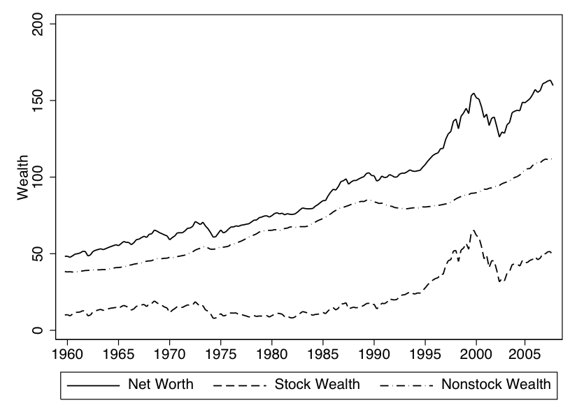
Note: Per capita real wealth figures in thousands of year 2000 dollars. Net worth is our measure of total wealth.
Ct = κBt + εt
| Estimated κ
| |||
| True κ | n = 20 | n = 40 | n = 60
|
| 0.0137 | -0.0486 | -0.0185 | -0.0082 |
Notes: Both variables normalized with permanent income Pt. “True κ’ =  R - (Rβ)1∕ρ
 ∕R.
Calibration: ρ = 2, β = 0.99, R = Gρ∕β, Π = 0.25, G = 1.0151∕4, G = 1.0251∕4, wealth shock
= 1.
∕R.
Calibration: ρ = 2, β = 0.99, R = Gρ∕β, Π = 0.25, G = 1.0151∕4, G = 1.0251∕4, wealth shock
= 1.
Δ t = χEt-2Δ
 t-1 + αΔ
 t-1 + εt
| Estimated
| |||||||
| True | n = 20 | n = 40 | n = 60
| ||||
| χ |  R - (Rβ)1∕ρ R - (Rβ)1∕ρ ∕R ∕R | χ | α∕χ(1 - χ) | χ | α∕χ(1 - χ) | χ | α∕χ(1 - χ)
|
| 0.75 | 0.694 | 0.724 | 0.734 | ||||
| 0.75 | 0.0137 | 0.698 | 0.0117 | 0.741 | 0.0136 | 0.751 | 0.0067 |
Notes: Calibration: ρ = 2, β = 0.99, R = Gρ∕β, Π = 0.25, G = 1.0151∕4, G = 1.0251∕4, wealth shock
= 1. Δ t-1 instrumented with Δ
 t-2.
t-2.
∂ t = α0 + α1
 t-1 + α2
 t-1f + α3
 t-1h + α4MUt-1 + α5FFt-1
| Next-Quarter Effect | Extra | |||||
| of $1 Change in Wealth | Variables | |||||
| Total | Financial | Housing | Unemp Exp | Fed Fund | Test of | |
 t-1 t-1 |  t-1f t-1f |  t-1h t-1h | MUt-1 | FFt-1 |  f = f =  h h | 2 |
| 0.017*** | 0.130 | |||||
| (0.004) | ||||||
| 0.009*** | 0.086*** | -0.399* | 0.222 | |||
| (0.003) | (0.032) | (0.209) | ||||
| 0.016*** | 0.039*** | 0.066 | 0.138 | |||
| (0.004) | (0.011) | |||||
| 0.008*** | 0.018** | 0.082** | -0.411* | 0.271 | 0.225 | |
| (0.003) | (0.008) | (0.034) | (0.211) | |||
Notes: Sample period is 1960Q1–2007Q4. Standard errors in parentheses. {*,**,***}=Statistical significance at {10, 5, 1} percent. Coefficients on wealth variables reflect MPCs in the quarter following a wealth change: For example, the coefficient 0.017 in the first row implies that a one dollar increase in wealth in the previous quarter translates into a 1.7 cent increase in consumption in the current quarter. The wealth variables are from the Flow of Funds balance sheets for the household sector. MU is the fraction of consumers who expect the unemployment rate to decline over the next year minus the fraction who expect it to increase. FF is the nominal Fed funds rate. The wealth and consumption variables were normalized by the level of consumption expenditures at t - 4 to correct for the long-term trends in consumption and wealth. The equations without the extra variables exhibited serial correlation and so standard errors for those equations are corrected for serial correlation using the Newey–West procedure with 4 lags.
∂ t+1 =
t+1 =  0 + χEt-1∂
 t + εt+1
| Variables used | Consumption Growth | Implied Eventual
| ||
| to forecast | Momentum Coefficient | MPC out of
| ||
Et-1∂ t t | χ | Total  | Financial  f f | Housing  h h |
 | 0.58** | 0.070 | ||
| (0.23) | ||||
 , , | 0.76*** | 0.048 | ||
| MU, FF | (0.14) | |||
 f, f, h h | 0.45** | 0.064 | 0.159 | |
| (0.20) | ||||
 f, f, h, h, | 0.71*** | 0.041 | 0.087 | |
| MU, FF | (0.13) | |||
Notes: Sample period is 1960Q1–2007Q4. Standard errors are in parentheses. {*,**,***} = Statistical significance at {10, 5, 1}
percent. The eventual MPCs are calculated from the formula αj∕χ(1 - χ) where αj is the corresponding next-quarter MPC
estimated in table 3. Standard errors for all equations are heteroskedasticity and serial-correlation robust. When more instruments
are used to forecast ∂ t (for example, interest rate spread and the change in unemployment over the previous year), the estimate
of χ tends to rise further and the standard error falls further. The measure of the change in wealth used for the regressions is the
∂
t (for example, interest rate spread and the change in unemployment over the previous year), the estimate
of χ tends to rise further and the standard error falls further. The measure of the change in wealth used for the regressions is the
∂ measure defined in the text, as this can be measured without an estimate of χ, unlike the
  measures used in the previous
table.
measures used in the previous
table.
| Immediate Effect | Eventual Effect | ||||||||
| of $1 Change in Wealth | of $1 Change in Wealth | ||||||||
| Total | Financial | Housing | Total | Financial | Housing | Test of | |||
| Model | χ | Bt-1 | Bt-1f | Bt-1h | Bt-1 | Bt-1f | Bt-1h | Bf = Bh | 2 |
| M1 | 0 .731*** | 0.013*** | 0.066 | 0.301 | |||||
| (0.149) | (0.005) | ||||||||
| M2 | 0.737*** | 0.011*** | 0.024** | 0.055 | 0.123 | 0.162 | 0.309 | ||
| (0.153) | (0.004) | (0.010) | |||||||
| M3 | 0.634*** | 0.015*** | 0.063 | 0.301 | |||||
| (0.199) | (0.006) | ||||||||
| M4 | 0.601*** | 0.013** | 0.028** | 0.053 | 0.116 | 0.187 | 0.307 | ||
| (0.197) | (0.005) | (0.012) | |||||||
| M5 | 0.741*** | 0.009*** | 0.047 | 0.223 | |||||
| (0.132) | (0.003) | ||||||||
| M6 | 0.719*** | 0.008*** | 0.018** | 0.041 | 0.087 | 0.273 | 0.224 | ||
| (0.131) | (0.003) | (0.008) | |||||||
| M7 | 0.855*** | 0.007*** | 0.022 | 0.060 | 0.176 | 0.309 | 0.119 | ||
| (0.148) | (0.002) | (0.014) | |||||||
Notes: Sample period is 1960Q1–2007Q4. Standard errors in parentheses. {*,**,***}=Statistical significance at {10,5,1} percent. Models M1 and M2 are estimated with an alternative instrument set which consists of growth rate of stock prices, change in unemployment rate, growth rate of disposable income and interest rate spread. Models M3 and M4 are estimated with lags t - 3 and t - 4 of these instruments. Models 5 and 6 are estimated using the iterative procedure described in section 3.5.