0.05 at an annual frequency (that
is, over the year following a $1 stimulus check, spending will be higher by 3 to 5
cents).1
0.05 at an annual frequency (that
is, over the year following a $1 stimulus check, spending will be higher by 3 to 5
cents).1
_____________________________________________________________________________________
Abstract
Today’s dominant strain of macroeconomic models supposes that aggregate
consumption can be understood by assuming the existence of a ‘representative
agent’ whose behavior rationalizes observed outcomes. But representative agent
models yield embarrassingly implausible (and empirically inaccurate)
descriptions of consumption behavior. When push comes to shove, real-world
forecasters (including those at the Fed) properly disregard these implications. As
a result, consumption forecasting remains very much a seat-of-the-pants
enterprise. I will argue that if the representative agent assumption is replaced
with a model that generates wealth heterogeneity that matches the empirical
data, the improved model can provide a sensible analysis of economic questions
like “What might the consumption response be to economic stimulus payments?”
Microfoundations, Wealth Inequality, Marginal Propensity to Consume
D12, D31, D91, E21
| PDF: | http://www.econ2.jhu.edu/people/ccarroll/papers/W-Hetero-Fed.pdf |
| Web: | http://www.econ2.jhu.edu/people/ccarroll/papers/W-Hetero-Fed/ |
| Archive: | http://www.econ2.jhu.edu/people/ccarroll/papers/W-Hetero-Fed.zip |
| BibTeX: | http://www.econ2.jhu.edu/people/ccarroll/papers/W-Hetero-Fed-Self.bib |
1Carroll: Department of Economics, Johns Hopkins University, Baltimore, MD, http://www.econ2.jhu.edu/people/ccarroll/, ccarroll@jhu.edu. This paper was written for an Academic Consultants’ meeting at the Board of Governors of the Federal Reserve System on May 14, 2012. Thanks to Jirka Slacalek and Kiichi Tokuoka; most of the results in this paper are taken from Carroll, Slacalek, and Tokuoka (2011).
Most modern macroeconomic models assume that aggregate consumption is
determined by a ‘representative agent’ whose spending decisions reflect aggregate
net worth and expectations about the future path of national income. Such models
invariably imply that spending is virtually unaffected by transitory shocks like
economic stimulus payments: The models imply that the ‘marginal propensity to
consume’ (MPC) is typically around 0.030.05 at an annual frequency (that
is, over the year following a $1 stimulus check, spending will be higher by 3 to 5
cents).1
This is an unfortunate prediction, because a literature dating back to the 1950s, ranging across countries and institutional arrangements, has found that transitory, or in Friedman (1963)’s terminology, ‘windfall,’ shocks, tend to have effects on spending that are much larger than 3 to 5 cents per dollar. Although Friedman is sometimes invoked as a progenitor of representative agent models, his considered judgment (cf. Friedman (1963)) was that the annual MPC was about 1/3.
Empirical evidence suggests that Friedman’s view was closer to the truth than either the original Keynesian view (with an MPC near one) or the modern representative agent view (with an MPC near zero). I will argue that the main reason that Friedman was right is because the (empirically observed) large differences in wealth across consumers imply large differences in MPC’s.
An example nicely illustrates the representative agent model’s error. Some years ago, undergraduates at the University of North Carolina choosing their major field of study were informed about the average post-graduation incomes of UNC graduates who had chosen to study in various fields. Surprisingly, the field that exhibited the highest average income was Geography. It turned out, however, that this was because Michael Jordan had been a Geography major. Roughly speaking, representative agent models make the same mistake most UNC undergraduates were probably smart enough to avoid: Supposing that the mean is a good measure of the object you are interested in.
Translating this point into the wealth-and-consumption arena, both theory and evidence suggest that the MPC is much higher for people with low levels of wealth than for the people at the top of the distribution. It may be true that a person with a wealth-to-income ratio of 4 or higher (matching the economy as a whole) would have an MPC not too different from 0.04. But if the economy consisted of 1 person with a wealth of 400 (and an MPC of 0.04) and 99 people with wealth of zero (and an MPC of 1), the aggregate MPC out of a transitory shock to income would only be 0.04 if the entire stimulus payment were made to this economy’s Michael Jordan.
The actual distribution of wealth is not so extreme as in this example. The bulk of my discussion will focus on teasing out the quantitative implications of empirical wealth data. The conclusion is that data from the Fed’s Survey of Consumer Finances (SCF) suggest that the aggregate MPC should be at the very least about 0.2 at an annual frequency (five times greater than in a representative agent model). If we assume that some forms of wealth (housing wealth, for example) are completely illiquid and therefore irrelevant for the exercise, a Friedmanesque model is capable of producing an annual MPC as high as 0.7. More plausible is an intermediate case, in which housing and other illiquid wealth is less accessible than a checking account but not entirely irrelevant for consumption decisions. Such a model would produce an intermediate MPC, which would likely fall somewhere in the range typically found in the empirical literature (say, ten times larger than the representative agent model implies). (“Likely,” because there is not yet a consensus on how to model illiquidity).
My focus on the MPC may seem a bit narrow. After all, many other questions about consumption dynamics are important in the medium run (most notably, the path of the personal saving rate). However, this narrow focus is motivated by deep theoretical considerations; the MPC pops up everywhere in theoretical analyses of household choice. For example, theory implies that the MPC is closely connected to risk aversion in portfolio choice; the response of labor supply to increased uncertainty; the extent to which knowledge about future taxes affects current spending; and many other questions.
Before we get to the theoretical framework, a brief discussion of the evidence on MPC’s is called for. After the evidence and the theory come some further implications for macroeconomic analysis and some conclusions.
Good evidence on average MPC’s is scant. This is because direct measurement of an MPC requires both extraordinary data and unusual circumstances. What is needed, ideally, is a microeconomic data source with high quality data on changes in individual households’ spending that can be related to ex-post clearly identifiable, but ex-ante unexpected, transitory shocks to income (‘windfalls’, in Friedman’s terminology, if the shock is positive).
Disaggregated data is essential, because any particular episode constitutes only a single macroeconomic datapoint. The impossibility of drawing statistically compelling conclusions from a one-off experiment has been illustrated by the recent debate between two Republican economists, John Taylor (2009) and Mark Zandi (2010), about the stimulus payments made by the George W. Bush administration in the spring of 2008.2 Taylor argues the stimulus failed because consumption spending shows no upsurge in the quarter when the stimulus payments were received. But Zandi (a ‘real world’ economist if ever there was one) notes that the checks arrived at a point when household wealth was falling precipitously, consumer confidence was plummeting, and credit availability was tightening; indeed, the gathering economic headwinds were precisely what motivated Congress and the President to enact the stimulus package. Zandi concludes that, without the stimulus payments, consumption would have dropped sharply. But whether Taylor or Zandi is right is statistically unanswerable using a single aggregate datapoint. The impossibility becomes even more obvious when the argument is recast in a more appropriate framework: The question at issue (for evaluating the effectiveness of short-run stimulus) is whether (and by how much) spending is higher some interval (such as a year) following the receipt of the windfall. If the effect within the quarter is statistically unknowable, the effect over the subsequent year is quadruply so.
If Congress were in the habit of passing (and Presidents of signing) large uniform ‘windfall’ tax cuts at random (that is, independently of the state of the economy), then over the course of a century or two we might accumulate sufficient macroeconomic data to reliably estimate a time path for their effects (assuming the MPC itself was stable over that century). But in practice, only a few clear-cut experiments exist, motivated in every case by perceptions of a weakening economy, and with widely different characteristics (George W. Bush’s 2008 package, for example, was clearly specified as a one-time ‘windfall’ tax cut, while George H.W. Bush’s 1990–91 plan merely involved rearranging the timing of tax payments; the Obama package was more complex and contained several elements. Its largest component will be discussed briefly below).
The principal U.S. source of microeconomic data on comprehensive household spending is the Consumer Expenditure Survey (the ‘CE’ survey for short) conducted by the Bureau of Labor Statistics. While the CE survey has serious and growing deficiencies (in some categories of spending, the survey’s estimate falls short of NIPA data by amounts ranging up to 50 percent), it is almost the only (microeconomic) game in town for these questions.
The first good opportunity to study these questions using CE data was provided by the 2001 stimulus payments of George W. Bush. In a heroic feat of bureaucratic agility, after the stimulus legislation passed the Bureau of Labor Statistics managed to add a few questions to the CE survey in time to permit researchers to identify the date at which each surveyed household received its stimulus check. Using these timing differences, Johnson, Parker, and Souleles (2006) estimated that the effect of receiving the check earlier rather than later implied that household spending on nondurable goods may have been boosted by the checks by about 50 cents on the dollar over the six months following receipt of the payments. (Using different data, Agarwal, Liu, and Souleles (2007) found similar results using credit card data.)
These results are difficult to evaluate, however, because it is not clear how households interpreted the stimulus checks in 2001, which were essentially an advance payment on future permanent tax cuts. In a model where households have perfect knowledge of the changes in their future taxes the instant the tax law changes and immediately reoptimize their spending accordingly, the proper interpretation of the 2001 checks is that they reflected a transitory movement of liquidity from the future to the present. But it seems at least as plausible that households with other things on their minds did not really realize that a ‘permanent’ tax cut had occurred until they received the letter and the check. In that case the documents may, at least to some households, have signaled a previously unnoticed shock to permanent income.
Friedman (1957) rightly emphasized long ago that the MPC out of transitory shocks should be much less than out of permanent shocks. As a result, under reasonable assumptions about households’ information, the 2001 episode can be interpreted either as demonstrating a higher-than-expected MPC out of transitory shocks or a lower-than-expected MPC out of permanent shocks.
A cleaner experiment was provided by the 2008 stimulus package. This event was explicitly designed as a pure transitory “windfall” payment to households. The uninformative solitary macroeconomic datapoint hotly debated by Taylor and Zandi manifests itself, in the CE survey, in almost 20,000 relevant microeconomic datapoints, because different households received their stimulus payments at different times; each household is observed over multiple periods; the amounts received varied depending on observable household characteristics; and those characteristics (e.g., wealth and income levels) can be used, as theory suggests, as conditioning variables for estimating MPCs.
Parker, Souleles, Johnson, and McClelland (2011) have estimated the effect of this payment at around 40 cents on the dollar in spending on nondurable goods and services over the subsequent 6 months, while the estimated effect on total spending was about 75 cents per dollar of stimulus payment received (owing largely to the fact that a small but statistically significant proportion of stimulus recipients used their checks as down payments for purchasing a vehicle). Parker, Souleles, Johnson, and McClelland (2011) estimate that the stimulus payments increased aggregate spending by between 1.3 and 2.3 percent in the second quarter of 2008 – and their estimate (unlike those of Taylor and Zandi) has statistically quantifiable significance.
These studies rank as the best available direct recent evidence on the size of MPC’s in the U.S. Over the years since Friedman (1957) first formulated the Permanent Income Hypothesis, a number of interesting special episodes have been examined for evidence of the size of the MPC, including one-time events like German reparations payments to Israeli citizens who suffered during the Holocaust (Kreinin (1961)). On the whole, these studies have tended to produce results consistent with annual MPC’s in the range of 0.2–0.7, with some hints that the MPC is lower when payments are larger.3
Generalizing across the entire literature since Friedman’s time, one robust conclusion that emerges repeatedly is that the marginal propensity to consume tends to be higher for households with lower levels of wealth. This is deeply unsurprising, as it is an implication of the concavity of the consumption function (that is, the higher MPC at lower levels of wealth) visible in figure 1 (and proven as a general feature of models of consumption under uncertainty by Carroll and Kimball (1996)).
A closely related literature has attempted to estimate the size of ‘wealth effects’ on consumption. Here, the question at issue is by how much spending changes following a shock either to financial wealth, or to housing prices, or to some other component of net worth. Particularly interesting is the work of Disney, Gathergood, and Henley (2010) which shows that in the U.K. the effect of house price shocks is sharply different across households with negative versus positive equity. But it is not clear ‘wealth effects’ studies of this kind provide reliable answers to questions like ‘what effect might stimulus payments have.’ What they do persuasively demonstrate, again, is the quantitative importance of heterogeneity across households in conditioning the aggregate response to a shock.
Evidence on all these questions is not more copious mainly because our data sources are highly problematic. But the questions are so important to the conduct of macroeconomic forecasting and monetary policy that the Federal Reserve would be amply justified in aggressively seeking ways of improving the data available to researchers. A question of particular importance for monetary policy is the marginal propensity to consume out of interest income; this is a complex topic, because changes in interest rates have a host of effects on spending, including channels involving credit availability, portfolio choice, and, theoretically, even labor supply. But very little good empirical evidence exists on any of these questions because of the inadequacy of the data sources. (Recognizing the importance of the question, the Bank of England has recently initiated a survey of consumers asking them direct questions designed to elicit consumers’ estimates of their own MPC’s; results have not been published yet, so whether the enterprise will succeed is unknown. But the attempt illustrates the importance that the BoE assigns to obtaining at least some glimmerings of empirical evidence on the subject).
The recent experiment with a panel version of the Survey of Consumer Finances is a very welcome move in the general direction of better micro measurement, and it is not unreasonable to hope that eventually even better measurement will be possible as wealth measurement technology progresses. So far as I know, nobody has yet attempted to construct estimates of the MPC from this data source (which only became available to the public a short time ago), but such an effort might prove very interesting.4
In principle, if high-quality data were available on regional (say, state-level or city-level) variation in income, spending, and the various components of wealth, differences in the regional distribution of economic shocks might be used to tease out reliable estimates of aggregate MPC’s.
Pioneering work by Case, Quigley, and Shiller (2005) (updated in Case, Quigley, and Shiller (2011)) attempted to address the related question of the relative size of ‘wealth effects’ on consumption from shocks to housing wealth and from stock market wealth. Severe data difficulties (in particular, the questionable quality of their state-level consumption and stock wealth data) may have initially deterred many macroeconomists from following in their footsteps.
Recently, however, work by Mian, Sufi, and collaborators has reinvigorated this approach, in part by finding new sources of data and in part by choosing to ask different questions. Most directly relevant is the paper of Mian, Rao, and Sufi (2011), who find that movements in housing prices are strongly associated with movements in local spending (using an extremely promising new data source on local spending from MasterCard Advisors). They show, among other things, that in the Great Recession consumption fell most in places where the prior buildup in housing-related debt had been greatest (a finding that the International Monetary Fund (2012) has recently shown holds for countries as well; Karen Dynan (2012) similarly finds that households whose house prices have fallen sharply experienced big declines in spending). These empirical results are very much along the lines of what might be expected from microeconomic models that incorporate the kinds of heterogeneity advocated here. While model with a proper treatment of the theoretical complexities involved in adding housing and debt has not yet been constructed, it is seems likely that it would be possible for such a model to explain the results of Mian, Rao, and Sufi (2011), Dynan (2012), and others. But what is perfectly clear is that those results cannot be plausibly explained in a representative agent model.
I will employ a standard “buffer stock” model of household behavior, in which individual households make their spending decisions knowing full well that they face substantial income uncertainty. The magnitude of that income uncertainty is calibrated to match facts from the microeconomic data (the most reliable source is newly-available Social Security earnings records; see Sabelhaus and Song (2010)).
Income  is assumed, following Friedman (1957), to have two components, a
transitory component (which would include windfalls like a one-time stimulus
check) and a permanent component that reflects earnings in a “normal”
year.
is assumed, following Friedman (1957), to have two components, a
transitory component (which would include windfalls like a one-time stimulus
check) and a permanent component that reflects earnings in a “normal”
year.
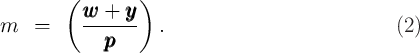
Because current spending can be financed either out of current income  or
out of past accumulated wealth
or
out of past accumulated wealth  , it is useful to combine those two variables a
single measure of the consumer’s spending power called ‘market resources’
, it is useful to combine those two variables a
single measure of the consumer’s spending power called ‘market resources’  :
:

In my model, a household’s consumption choice is determined by the ratio of
its market resources to its permanent income,  . Using non-boldface letters to
indicate variables that have been scaled by permanent income, the ratio of
consumption to permanent income,
. Using non-boldface letters to
indicate variables that have been scaled by permanent income, the ratio of
consumption to permanent income,  , is determined by the ratio of market
resources to permanent income:
, is determined by the ratio of market
resources to permanent income:
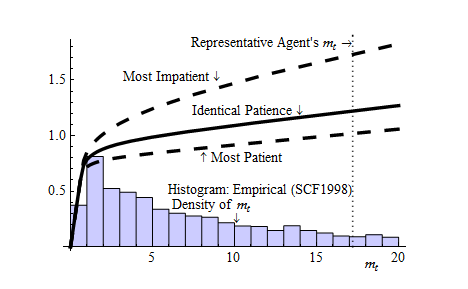
In the presence of uncertainty and under the assumption (“Identical
Patience”) that all households have identical target levels of wealth, a
version of the model calibrated to match the total amount of wealth in the
U.S. economy implies a relationship between consumption spending and
household  shown as the thick solid curve labeled “Identical Patience” in
figure 1.5
(The label, the dashing curves, and the histogram will be explained shortly).
shown as the thick solid curve labeled “Identical Patience” in
figure 1.5
(The label, the dashing curves, and the histogram will be explained shortly).
The marginal propensity to consume out of an additional (transitory)
dollar of income is simply the amount by which consumption increases as
 increases. At low values of wealth, the relationship is very steeply
sloped, with a near-Keynesian MPC close to 1. At large values of wealth,
the slope is much flatter, and indeed theoretical analysis shows that as
increases. At low values of wealth, the relationship is very steeply
sloped, with a near-Keynesian MPC close to 1. At large values of wealth,
the slope is much flatter, and indeed theoretical analysis shows that as
 gets to the vicinity of the aggregate value of the wealth-to-income
ratio (labelled as “Representative agent’s
gets to the vicinity of the aggregate value of the wealth-to-income
ratio (labelled as “Representative agent’s  ”), the MPC is close to
the 0.04 (at an annual frequency) implied by the representative agent
model.
”), the MPC is close to
the 0.04 (at an annual frequency) implied by the representative agent
model.
(The representative agent’s  value is shown as about 16; but remember that
the measure of income we are considering is quarterly; so an
value is shown as about 16; but remember that
the measure of income we are considering is quarterly; so an  of 16
corresponds to a wealth-to-annual-income ratio of about 4. Because annual
MPC’s are more intuitive than quarterly ones, we translate our quarterly MPC’s
into annual rates, so the annual MPC of 0.04 mentioned above corresponds to a
quarterly MPC of about 0.01.)
of 16
corresponds to a wealth-to-annual-income ratio of about 4. Because annual
MPC’s are more intuitive than quarterly ones, we translate our quarterly MPC’s
into annual rates, so the annual MPC of 0.04 mentioned above corresponds to a
quarterly MPC of about 0.01.)
Plotted as a histogram on the same figure is data from the 1998 SCF on the empirical
distribution of wealth.6
The economywide MPC should reflect a weighted average of the MPC’s at the
different values of  , where the weights reflect the proportion of households
observed holding each different value of
, where the weights reflect the proportion of households
observed holding each different value of  .
.
The histogram shows that, in the empirical wealth data, a large proportion of
households have a  ratio close to 1. (Recall that income itself is included in
 so a value of 1 would characterize a consumer with wealth of zero
((wealth
so a value of 1 would characterize a consumer with wealth of zero
((wealth income)/income)
 1). To many macroeconomists unfamiliar with
the micro data, the fact that so many households have so little wealth sometimes
comes as a shock; but it is a robust fact that emerges not only from all the
successive waves of the SCF, but from every other micro data source that
attempts to measure wealth. (A striking fact from Lusardi, Schneider, and
Tufano (2011) is that about a quarter of Americans report that in case of an
emergency need for cash, they would not be able to come up with $2000 in 30
days.)
1). To many macroeconomists unfamiliar with
the micro data, the fact that so many households have so little wealth sometimes
comes as a shock; but it is a robust fact that emerges not only from all the
successive waves of the SCF, but from every other micro data source that
attempts to measure wealth. (A striking fact from Lusardi, Schneider, and
Tufano (2011) is that about a quarter of Americans report that in case of an
emergency need for cash, they would not be able to come up with $2000 in 30
days.)
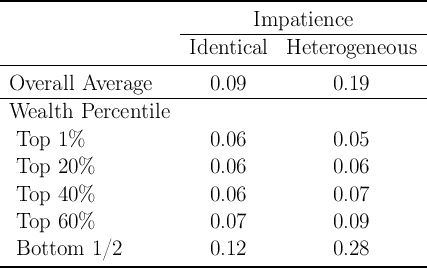
Table 1 computes the aggregate annual MPC that emerges from a model of this kind which is calibrated in such a way that the total level of aggregate net worth matches observed net worth in the U.S. economy. The first column of the table, labeled “Identical Impatience,” indicates that the model implies an aggregate MPC of only 0.09. While this is bigger than the 0.04 implied by the representative agent model, it remains far below the empirical estimates cited above.
The main reason this baseline model fails to produce much of an increase in the MPC is that it fails to match the degree of inequality empirically observed in the wealth distribution (visible in the histogram in the figure).
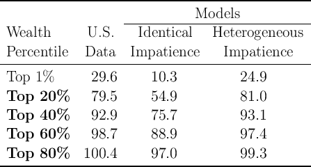
This point is illustrated by table 2, which shows the proportion of aggregate wealth held by households in the top 1 percent, top 10 percent, and other net worth percentiles in the model and in the SCF data. For example, the first row shows that the model implies that the richest 1 percent of households should own only about 10 percent of aggregate net worth, while the data shows them actually holding about 30 percent.
The reason the wealth distribution is so equal (in the model) is that income shocks are the only reason households differ from each other. A more realistic model would allow for differences in age, in expected income growth, family size, and in a host of other factors that could lead different households to have different wealth targets.
Within the model, the simplest mechanism for generating different wealth targets across households is to permit households to differ in their degree of patience. This should not be interpreted literally; instead, differences in “patience” in the context of the model are a simple way to proxy for the large suite of characteristics (age, etc) that in the real world make households differ in their target wealth values.
The next column of table 2 shows the results when we allow households to have different degrees of patience, and ask the computer to find the heterogeneity in patience that makes the model best match the SCF wealth data at the 20th, 40th, 60th, and 80th percentiles.7 As the table shows, the model is now able to match these targeted points (typeset in bold face in the table) in the wealth distribution quite well, even at the tenth percentile which was not explicitly targeted. The model still somewhat underestimates the accumulation of wealth in the top 1 percent, but this is likely because the model does not incorporate entrepreneurial activity, which is the source of much of the wealth of the richest households. (The consumption functions that characterize the most patient and the least patient households in this modified version of the model are shown as the dashed lines in figure 1).
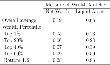
With greater wealth heterogeneity, the model produces a higher average annual MPC, now around 0.2 (the second column in table 3). This approaches the range of empirical estimates (though at the very low end). But we can go further. Recall that our exercise was to match the distribution of total net worth in the population. Implicitly, this assumes that all wealth is equally liquid and available for financing consumption at any instant. In reality, some forms of wealth are considerably more illiquid than others; if consumers find it difficult to spend out of the net worth tied up in illiquid assets, the appropriate measure of wealth for the model to match may be some more liquid measure of wealth.
The assumption at the opposite extreme from matching total net worth would be to ask the model to match the distribution of liquid (financial) assets, ignoring illiquid assets altogether for purposes of computing the MPC.8 Results of that exercise are presented in table 3.
The degree of inequality in liquid assets is much greater than that in total net worth; as a number of papers have emphasized recently (including Hall (2011) in his AEA Presidential Address), many households have remarkably small amounts of liquid assets. In order to match this fact, the model must assume that, with respect to their decisions about liquid assets, many households exhibit a high degree of impatience. (This might be justified, for example, in a model of the kind pioneered by Laibson (1997), if household deliberately segregate assets into illiquid and liquid forms in part for self-control reasons).
When we ask our model to match data on liquid assets, over a quarter of
households now have an  of less than 2. (That is, (income+wealth)/income is
less than 2, so wealth/income is less than 1). As a result of the high degree of
impatience needed to match the observed holdings of liquid assets, the model
now implies that the aggregate average MPC is almost 0.7—much higher than
the 0.2 that emerged from the model that (effectively) treated all assets as
liquid.
of less than 2. (That is, (income+wealth)/income is
less than 2, so wealth/income is less than 1). As a result of the high degree of
impatience needed to match the observed holdings of liquid assets, the model
now implies that the aggregate average MPC is almost 0.7—much higher than
the 0.2 that emerged from the model that (effectively) treated all assets as
liquid.
Neither of these models is entirely reasonable. Because illiquidity surely has some importance, it is not surprising that the first model somewhat underestimates the empirical MPC out of a transitory shock to income (which is by definition an increment to liquid, not illiquid, resources). But households do have some ability to tap illiquid assets when needed, so the second model (which ignores illiquid assets altogether) is also implausible. An intermediate case, with a formal treatment of the nature of illiquidity, would surely produce estimates between the 0.2 and 0.7 extremes computed in the two special cases. (See Kaplan and Violante (2011) for an interesting attempt to grapple with the intermediate case). The likely result from any intermediate model would be an MPC comfortably within the range of empirical estimates.
The perspective presented here about how to model consumption has a number of implications for the analysis of spending responses to both fiscal and monetary policy.
The most obvious is that the effects of a policy will depend not just on its total impact on aggregate income, but on how that effect is distributed across households with different MPC’s. But the Congressional Budget Office, the Office of Management and Budget, and the Treasury regularly prepare assessments of the distributional effects of tax policies, based on microsimulation models; the Federal Reserve undoubtedly has the resources and capacity to follow suit.
Just as important is the point that (as Friedman asserted long ago) the consumption response to an income shock should depend mightily on whether that change is perceived to be transitory or permanent, with responses to permanent changes expected to be much larger than for transitory changes. Unfortunately, no currently available data source is useful in measuring households’ perceptions of the degree to which given changes in their income are transitory or permanent, so this implication of Friedman’s framework has been difficult to test.
A good example of the practical complexities here comes from the Obama administration’s “Making Work Pay” tax reductions. The tax change took the form of a reduction for (at first) two years in the proportion of workers’ wages that were withheld for Social Security. This tax cut has since been extended, and may be extended again. But according to the theory employed above, households’ responses to these tax changes should depend on whether they perceive this as a permanent or as a transitory tax cut. (Or, indeed, whether they perceived it at all; some analysts have argued that because the tax change was not visibly manifested in the form of a check and a letter from the IRS, many households may not have perceived the tax cut, though they presumably noticed the extra money in their bank accounts. See Sahm, Shapiro, and Slemrod (2010) for a discussion of possible consequences of the method of delivery of the Obama stimulus payments).
The inability to answer questions like this using any available data source represents a serious gap in our ability to analyze fiscal policy, second in importance only to our ignorance about the effects of monetary policy at the household level (in large part reflecting ignorance about the distribution of those effects). There is some reason to hope that eventually a redesigned version of the CE survey will be better able to shed light on these and other questions, or that continuation of the SCF panel will permit better analysis. And cooperation or coordination between the SCF group at the Fed and the CE group at the BLS, particularly during the crucial period of CE redesign now commencing, could pay large long-term dividends. But there can be little doubt that current knowledge is woefully inadequate, given the importance of the questions.
In the wake of the Great Recession, withering criticism has been leveled at the state of macroeconomic modeling. During the crisis, the dominant class of models, representative agent Dynamic Stochastic General Equilibrium (DSGE) models, either had nothing useful to say about the policy questions that urgently needed answers (like how to respond to a financial panic), or provided answers sharply at variance with both common sense and empirical evidence (e.g., what to expect for the marginal propensity to consume out of economic stimulus payments). Fortunately, at least in the U.S., the these models were mostly ignored by policymakers savvy enough to see that they did not make sense. (See, e.g., Martin Wolf’s interview with Lawrence Summers (2011) for the Financial Times.9 ).
Given this history, it is hard not to sympathize with Krugman (2009)’s description of the current state of macroeconomics as a new dark age, in which hard-won wisdom (from sources as varied as Milton Friedman and John Maynard Keynes) has been tossed aside in pursuit of a gratuitous theological purity. But historians sometimes argue that developments during the historical dark ages laid the foundations for the scientific revolution. My sense is that the same will eventually be said of the macroeconomic dark ages. Models will be rebuilt on foundations that explicitly incorporate heterogeneity, because it is impossible to sensibly study subjects like finance (how can the representative agent be subject to problems of asymmetric information?), fiscal policy (how do transfers across people with different MPC’s affect the economy?), and monetary policy (what effects do interest rates have when some people are borrowers and some are lenders?) without heterogeneity. And foundations for rigorous study of such questions have indeed been laid during this dark age, for example in the theoretical work of Stiglitz, Akerlof, Bernanke, Gertler, and Gilchrist (1996), and others, and in empirical work by a host of scholars who have mined microeconomic data for its macroeconomic insights over the past 30 years.
On those foundations, the task ahead is to build an edifice that is reasonably consistent with the best evidence available from whatever source (microeconomic, regional, or macroeconomic). In a great many cases, the “best evidence” cannot be macroeconomic, because so little macroeconomic data exist (as illustrated by the dispute about a single datapoint between Taylor and Zandi cited above). Wherever possible, macroeconomists will have to learn to calibrate and evaluate their models not only by their (often virtually untestable) implications for macroeconomic outcomes but also by whether the observable implications for relevant microeconomic quantities (such as the distribution of wealth) make sense.
With modern comptational power, this ambition is entirely feasible. But fulfilling it will require a renewed commitment of macroeconomists to the kind of microeconomic analysis that Friedman (1957), Modigliani and Brumberg (1954), and other macroeconomists pioneered long ago but that has not been the dominant fashion during the now-concluding dark age.
AGARWAL, SUMIT, CHUNLIN LIU, AND NICHOLAS S. SOULELES (2007): “The Reaction of Consumer Spending and Debt to Tax Rebates–Evidence from Consumer Credit Data,” Discussion paper, National Bureau of Economic Research, http://www.nber.org/papers/w13694.
BERNANKE, BENJAMIN, MARK GERTLER, AND SIMON GILCHRIST (1996): “The Financial Accellerator and the Flight to Quality,” Review of Economics and Statistics, 78, 1–15.
CARROLL, CHRISTOPHER D., AND MILES S. KIMBALL (1996): “On the Concavity of the Consumption Function,” Econometrica, 64(4), 981–992, http://www.econ2.jhu.edu/people/ccarroll/concavity.pdf.
CARROLL, CHRISTOPHER D., JIRI SLACALEK, AND KIICHI TOKUOKA (2011): “Digestible Microfoundations: Buffer Stock Saving in a Krusell-Smith World,” Manuscript, Johns Hopkins University, At http://www.econ2.jhu.edu/people/ccarroll/papers/BSinKS.pdf.
CASE, KARL E., JOHN M. QUIGLEY, AND ROBERT J. SHILLER (2005): “Comparing Wealth Effects: The Stock Market Versus the Housing Market,” Advances in Macroeconomics, 5(1), 1–32.
__________ (2011): “Wealth Effects Revisited 1978-2009,” Cowles Foudation Discussion Paper 1784, Cowles Foundaion for Reserch in Economics, Yale University.
DELONG, J. BRADFORD (2012): “This Time, It Is Not Different,” Rethinking Finance: Perspectives on the Crisis, http://www.russellsage.org/rethinking-finance.
DISNEY, RICHARD, JOHN GATHERGOOD, AND ANDREW HENLEY (2010): “House Price Shocks, Negative Equity, and Household Consumption in the United Kingdom,” Journal of the European Economic Association, 8(6), 1179–1207.
DYNAN, KAREN E. (2012): “Is Household Debt Overhang Holding Back Consumption?,” Brookings Papers on Economic Activity, http://www.brookings.edu/~/media/Files/Programs/ES/BPEA/2012_spring_bpea_papers/2012_spri.
FRIEDMAN, MILTON A. (1957): A Theory of the Consumption Function. Princeton University Press.
__________ (1963): “Windfalls, the ‘Horizon,’ and Related Concepts in the Permanent Income Hypothesis,” in Measurement in Economics, ed. by Carl Christ, pp. 1–28. Stanford University Press.
HALL, ROBERT E. (2011): “The Long Slump,” AEA Presidential Address, ASSA Meetings, Denver.
INTERNATIONAL MONETARY FUND (2012): World Economic Outlook, 2012chap. 3. International Monetary Fund, Available at http://www.imf.org/external/pubs/ft/weo/2012/01/pdf/text.pdf.
JAPPELLI, TULLIO, AND LUIGI PISTAFERRI (2010): “The Consumption Response to Income Changes,” Annual Reviews of Economics, 2(1), 479–506.
JOHNSON, DAVID S., JONATHAN A. PARKER, AND NICHOLAS S. SOULELES (2006): “Household Expenditure and the Income Tax Rebates of 2001,” American Economic Review, 96(5), 1589–1610.
KAPLAN, GREG, AND GIOVANNI L. VIOLANTE (2011): “A Model of the Consumption Response to Fiscal Stimulus Payments,” NBER Working Paper Number W17338.
KREININ, MORDECAI E. (1961): “Windfall Income and Consumption: Additional Evidence,” American Economic Review, 51, 388–390.
KRUGMAN, PAUL (2009): “A Dark Age of Macroeconomics,” http://krugman.blogs.nytimes.com/2009/01/27/a-dark-age-of-macroeconomics-wonkish/.
LAIBSON, DAVID (1997): “Golden Eggs and Hyperbolic Discounting,” Quarterly Journal of Economics, CXII(2), 443–477.
LUSARDI, ANNAMARIA, DANIEL J. SCHNEIDER, AND PETER TUFANO (2011): “Financially Fragile Households: Evidence and Implications,” NBER Working Paper Number 17072, (17072), http://www.nber.org/papers/w17072.
MAYER, THOMAS (1972): Permanent Income, Wealth, and Consumption. University of California Press, Berkeley.
MIAN, ATIF, KAMALESH RAO, AND AMIR SUFI (2011): “Household Balance Sheets, Consumption, and the Economic Slump,” Manuscript, University of California at Berkeley.
MODIGLIANI, FRANCO, AND RICHARD BRUMBERG (1954): “Utility Analysis and the Consumption Function: An Interpretation of Cross-Section Data,” in Post-Keynesian Economics, ed. by Kenneth K. Kurihara, pp. 388–436. Rutgers University Press, New Brunswick, N.J.
PARKER, JONATHAN A., NICHOLAS S. SOULELES, DAVID S. JOHNSON, AND ROBERT MCCLELLAND (2011): “Consumer Spending and the Economic Stimulus Payments of 2008,” NBER Working Paper Number W16684.
ROMER, CHRISTINA D. (2011): “What Do We Know about the Effects of Fiscal Policy? Separating Evidence from Ideology,” Speech at Hamilton College, November.
SABELHAUS, JOHN, AND JAE SONG (2010): “The Great Moderation in Micro Labor Earnings,” Journal of Monetary Economics, 57(4), 391–403, http://ideas.repec.org/a/eee/moneco/v57y2010i4p391-403.html.
SAHM, CLAUDIA R., MATTHEW D. SHAPIRO, AND JOEL SLEMROD (2010): “Check in the Mail or More in the Paycheck: Does the Effectiveness of Fiscal Stimulus Depend on How It Is Delivered?,” FEDS Working Paper No. 2010-40.
SHAPIRO, MATTHEW D., AND JOEL SLEMROD (2009): “Did the 2008 Tax Rebates Stimulate Spending?,” Manuscript, University of Michigan, http://www-personal.umich.edu/~shapiro/papers/Rebate2008-2008-12-27-assa-draft.pdf.
SUMMERS, LAWRENCE H. (2011): “Larry Summers and Martin Wolf on New Economic Thinking,” Financial Times video interview, http://tinyurl.com/dl201108a.
TAYLOR, JOHN B. (2009): “The Lack of an Empirical Rationale for a Revival of Discretionary Fiscal Policy,” The American Economic Review, 99(2), 550–555.
ZANDI, MARK (2010): “Perspectives on the Economy,” Testimony before the House Budget Committee, July 1.
 Distribution (ratios to quarterly income)