grows by a constant factor
  every period, reflecting exogenous
labor productivity improvements:
every period, reflecting exogenous
labor productivity improvements:
beginCDC
This handout illustrates the logic of precautionary saving by assuming that individuals face only a single, simple kind of uncertainty: A small risk of becoming permanently unemployed. More realistic assumptions yield similar conclusions (after much more work).1
The aggregate wage grows by a constant factor every period, reflecting exogenous
labor productivity improvements:
 | (1) |
The consumer lives in a small open economy – there is a constant interest factor  .
Defining
.
Defining  as market resources (net worth plus current income),
  as end-of-period assets
after all actions have been accomplished (specifically, after the consumption decision), and
as end-of-period assets
after all actions have been accomplished (specifically, after the consumption decision), and  as bank balances before receipt of labor income, the dynamic budget constraint (DBC) can be
decomposed into the following elements:
as bank balances before receipt of labor income, the dynamic budget constraint (DBC) can be
decomposed into the following elements:
 | (2) |
where  measures the consumer’s labor productivity (‘endowment’) and
  is a dummy variable indicating the consumer’s employment state: Everyone
is either employed (state ‘e’), in which case
is a dummy variable indicating the consumer’s employment state: Everyone
is either employed (state ‘e’), in which case  , or unemployed (state
‘u’), in which case
, or unemployed (state
‘u’), in which case  , so that for unemployed individuals labor income is
zero.2
, so that for unemployed individuals labor income is
zero.2
Once a person becomes unemployed, that person can never become employed
again (i.e. if  then
then  ). Consumers have a CRRA felicity
function3
). Consumers have a CRRA felicity
function3
 , and they discount future felicity geometrically by
  per
period.
per
period.
The solution to the unemployed consumer’s optimization problem is4
 | (3) |
where the  superscript signifies the consumer’s (un)employment status;
  is the marginal propensity to consume for the perfect foresight consumer,
which is strictly below the MPC for the problem with uncertainty (Carroll and
Kimball (1996)); and
is the marginal propensity to consume for the perfect foresight consumer,
which is strictly below the MPC for the problem with uncertainty (Carroll and
Kimball (1996)); and  is what Carroll (2022) calls the ‘return patience
factor.’5
is what Carroll (2022) calls the ‘return patience
factor.’5
We now impose the ‘return impatience condition’ (RIC),
 | (4) |
which deserves its name because it is the condition that guarantees that  – the consumer
must not be so patient that, given the interest rate, a boost to resources fails to boost
spending.6
An alternative (equally correct) interpretation is that the condition
guarantees that the PDV of consumption for the unemployed consumer is not
infinity.7
– the consumer
must not be so patient that, given the interest rate, a boost to resources fails to boost
spending.6
An alternative (equally correct) interpretation is that the condition
guarantees that the PDV of consumption for the unemployed consumer is not
infinity.7
For many purposes (not least, the calibration of the model), it turns out to be useful to
alternatviely express impatience conditions like (4) in terms of the upper bound of the range
of time preference factors  that satisfy the condition; solving (4) for
  , we designate this
object
, we designate this
object
 | (5) |
and write the alternative version of the constraint as
 | (6) |
 is the ‘return patience factor’ because it defines the patience factor
  relative
to the return factor
relative
to the return factor  ; correspondingly, we define the ‘return patience rate’ as
lower-case
; correspondingly, we define the ‘return patience rate’ as
lower-case
 | (7) |
and we say that a consumer is ‘return impatient’ if the RIC (4) holds (equivalent conditions are  and
and  ).8
).8
If a person who is employed in period  (
( ) is still employed next period (
 ),
market resources will be
),
market resources will be
 | (8) |
But employed consumers face a constant risk  of becoming unemployed. It will be convenient
to define
of becoming unemployed. It will be convenient
to define  as the probability that a consumer does not become unemployed.
Whether the consumer is employed or not, the consumer’s labor productivity
as the probability that a consumer does not become unemployed.
Whether the consumer is employed or not, the consumer’s labor productivity  is
well-defined:9
For convenience,
is
well-defined:9
For convenience,  is assumed to grow by a factor
  every period,
 | (9) |
which means that for a consumer who remains employed, labor income will grow by factor
 | (10) |
so that the expected labor income growth factor for employed consumers is the same  as in
the perfect foresight case:
as in
the perfect foresight case:
![( )
ℓtGWt
𝔼t[Wt+1 ℓt+1ξt+1] = ------- (℧ × 0 + //℧ × 1)
( ) //℧
𝔼t[Wt+1-ℓt+1-ξt+1]
Wt ℓt = G,](TractableBufferStock54x.svg) |
which is the reason for (9)’s assumption about the growth of individual labor productivity: It
implies that an increase in  is a pure increase in uncertainty with no effect on the PDV of
expected labor income (‘human wealth’); an increase in
is a pure increase in uncertainty with no effect on the PDV of
expected labor income (‘human wealth’); an increase in  therefore constitutes a
‘mean-preserving spread’ in human wealth.
therefore constitutes a
‘mean-preserving spread’ in human wealth.
The same solution methods used in PerfForesightCRRA can be applied here too (take
the first order condition with respect to  , use the Envelope theorem); the only
difference is the need to keep the expectations operator in place. Using
, use the Envelope theorem); the only
difference is the need to keep the expectations operator in place. Using  as a
placeholder for ‘e’ or ‘u,’ the usual steps lead to the standard consumption Euler
equation:
as a
placeholder for ‘e’ or ‘u,’ the usual steps lead to the standard consumption Euler
equation:
![[ ]
u′(cet) = R β 𝔼t u′(c∙t+1)
[( ∙ ) −ρ]
1 = R β 𝔼 ct+1 .
t cet](TractableBufferStock59x.svg) | (11) |
Defining nonbold variables as the bold equivalent divided by the level of permanent labor
income for an employed consumer, e.g.  , we can rewrite the consumption
Euler equation as
, we can rewrite the consumption
Euler equation as
![[ ]
( c∙ W ℓ ) −ρ
1 = R β 𝔼t -t+1--t+1-t+1-
cetWt ℓt
[( ∙ ) −ρ]
ct+1Φ
= R β 𝔼t cet ΦΦ
[( ) ]
−ρ c∙t+1 −ρ
= ΦΦΦ R β 𝔼t --e-
{ ct }
( ce )− ρ ( cu ) −ρ
= ΦΦΦ −ρR β (1 − ℧ ) -t+1- + ℧ -t+1
cet cet](TractableBufferStock61x.svg) | (12) |
It will be useful now to define a ‘growth patience factor’ (terminology justified below):
 | (13) |
which is the factor by which  would grow in the perfect foresight version of the model with
permanent income growth factor
would grow in the perfect foresight version of the model with
permanent income growth factor  (again see PerfForesightCRRA). Using this, (12) can be
written as
(again see PerfForesightCRRA). Using this, (12) can be
written as
![( e )− ρ{ [( u ) ( e ) ]−ρ}
1 = ÞÞÞρ ct+1- (1 − ℧) + ℧ ct+1 -ct-
ΦΦΦ cet cet cet+1
( )− ρ{ [( ) −ρ ]}
ρ cet+1- cut+1
= ÞÞÞΦΦΦ ce 1 + ℧ ce − 1
( ) { t [( ) ]t}+1
cet+1 ρ ρ cet+1- ρ
ce = ÞÞÞΦΦΦ 1 + ℧ cu − 1
( t ) { [( t+1 ) ]}
cet+1 cet+1- ρ 1∕ρ
ce = ÞÞÞΦΦΦ 1 + ℧ cu − 1 .
t t+1](TractableBufferStock65x.svg) | (14) |
beginCDC An interesting thought: Imagine the creation of an insurance system in which the
consumer pledges their next period  to the insurance company in exchange for receiving
a lognormally distributed
to the insurance company in exchange for receiving
a lognormally distributed  with an amount of variation that is (according to some
metric that deserves further thought) equivalent,
with an amount of variation that is (according to some
metric that deserves further thought) equivalent, ![e e 2 2
logˆct+1 ∼ 𝒩 (𝔼t[ct+1] − σˆct+1∕2,σ ˆct+1∕2)](TractableBufferStock68x.svg) .
In that case we would be able to compute analytically the value of
.
In that case we would be able to compute analytically the value of ![𝔼t[(cet+1)−ρ]](TractableBufferStock69x.svg) in (12) and
might be able to proceed with solving a version of the model with transitory as well as
permanent shocks.
in (12) and
might be able to proceed with solving a version of the model with transitory as well as
permanent shocks.
Second thoughts on this: This approach misses the concavity of the consumption function,
which may or may not matter much depending on the magnitude of the shocks. If it does
matter, it should be possible for the insurance company to provide a contract in which the
amount of consumption provided in the contract is, say, ∙](TractableBufferStock70x.svg) where
where  is lognormal
and
is lognormal
and  gives the best approximation to the slope of the consumption function around
![e
𝔼t[ct+1]](TractableBufferStock73x.svg) . How many people would buy the contract would depend on the profit
margin required by the insurance company, as well as consumption concavity. endCDC
. How many people would buy the contract would depend on the profit
margin required by the insurance company, as well as consumption concavity. endCDC
(This is where the perfect foresight assumption is important; without it (14) would be
![[ ( e ) −ρ { [ ( u )− ρ ] } ]
1 = ÞÞÞ ρ 𝔼 ct+1 1 + ℧ ct+1- − 1
ΦΦΦ t cet cet+1](TractableBufferStock74x.svg) | (15) |
and we would be unable to proceed.)
Now define  (which is the proportion by which consumption would be
greater next period for an employed than for an unemployed person), and define an ‘excess
prudence’ factor
(which is the proportion by which consumption would be
greater next period for an employed than for an unemployed person), and define an ‘excess
prudence’ factor
 | (16) |
Appendix A shows that, with some approximations, we can rewrite (11) as
 | (17) |
which can be simplified in the logarithmic utility case (where  ) to
) to
 | (18) |
Now since consumption if employed  is surely greater than consumption if unemployed
 ,
,  is certainly a positive number. But since
  is the value that
  would
exhibit in a perfect foresight model, this equation tells us that uncertainty boosts consumption
growth10 –
in the logarithmic case, consumption growth is augmented by an amount proportional to the
probability of becoming unemployed
would
exhibit in a perfect foresight model, this equation tells us that uncertainty boosts consumption
growth10 –
in the logarithmic case, consumption growth is augmented by an amount proportional to the
probability of becoming unemployed  multiplied by the size of the ‘consumption risk’ (the
amount by which consumption would fall if unemployment occurs).
multiplied by the size of the ‘consumption risk’ (the
amount by which consumption would fall if unemployment occurs).
We noted above that for any given  , an increase in uncertainty constitutes
a mean-preserving spread in human wealth; thus the ‘human wealth effect’ of an
increase in
, an increase in uncertainty constitutes
a mean-preserving spread in human wealth; thus the ‘human wealth effect’ of an
increase in  would be zero for a consumer without a precautionary motive. In this
small-open-economy model a change in
would be zero for a consumer without a precautionary motive. In this
small-open-economy model a change in  also has no effect on the interest rate
  , and so
none of the conventional determinants of consumption in the perfect foresight model
(the income, substitution, and human wealth effects) is affected by a change in
uncertainty. The increase in consumption growth from an increase in
, and so
none of the conventional determinants of consumption in the perfect foresight model
(the income, substitution, and human wealth effects) is affected by a change in
uncertainty. The increase in consumption growth from an increase in  in (17) or (18)
therefore must be entirely the result of the precautionary motive. Furthermore, because
a profile with faster consumption growth can only exhibit the same PDV if that
faster growth starts from a lower initial consumption level, we know that for any
given initial value of
in (17) or (18)
therefore must be entirely the result of the precautionary motive. Furthermore, because
a profile with faster consumption growth can only exhibit the same PDV if that
faster growth starts from a lower initial consumption level, we know that for any
given initial value of  , the introduction of a risk of becoming unemployed
  induces a (precautionary) decline in consumption (and corresponding increase in
saving).
induces a (precautionary) decline in consumption (and corresponding increase in
saving).
Furthermore, under the (compelling) assumption that  , (17) implies that a consumer
with a higher degree of prudence (larger
, (17) implies that a consumer
with a higher degree of prudence (larger  and therefore larger
  ) will anticipate a greater
increment to consumption growth as a consequence of the introduction of uncertainty.
This reflects the greater precautionary saving motive induced by a higher degree of
prudence.
) will anticipate a greater
increment to consumption growth as a consequence of the introduction of uncertainty.
This reflects the greater precautionary saving motive induced by a higher degree of
prudence.
The target level of  (if one exists) will be the point of intersection between the
  and
and  loci.
loci.
The  locus can be characterized by substituting
  :
:
![{ [( cet+1 )ρ ]} ρ
1 = 1 + ℧ -u-- − 1 ÞÞÞ ΦΦΦ
ct+(1 )
−ρ -ce- ρ
ÞÞÞ ΦΦΦ = (1 − ℧) + ℧ cu
( ) ( ) t+1
ÞÞÞ −ΦΦΦρ − 1 + ℧ 1∕ρ ce
------------- = -u--
◟-------℧◝◜-------◞ ct+1
≡ Π
( ≡ϖ ) 1∕ρ ( )
◜-−1-◞◟−ρ----◝ ce
( ℧ (ÞÞÞΦΦΦ − 1)+1 ) = -u--
ct+1
◟---------◝◜----------◞
Π=(1+ϖ)1∕ρ](TractableBufferStock101x.svg) |
which boils down to
 | (19) |
The importance of the linearity of the consumption function of the unemployed consumer
now becomes evident: It means that the RHS of (19) is linear in  :
:
 | (20) |
beginCDC
 | (21) |
and even if we had a solution for  , this equation defines the consumption function for the
employed consumer only implicitly; this explains why the linearity of the consumption
function for the unemployed consumer is essential for the tractability of the solution. endCDC
, this equation defines the consumption function for the
employed consumer only implicitly; this explains why the linearity of the consumption
function for the unemployed consumer is essential for the tractability of the solution. endCDC
We know that  because a consumer in these circumstances (facing possible
perpetual unemployment) will never borrow (see below for a full discussion of this point).
Since the RIC imposes
because a consumer in these circumstances (facing possible
perpetual unemployment) will never borrow (see below for a full discussion of this point).
Since the RIC imposes  , (20) tells us that steady-state consumption (if it
exists)11 is a positive finite
number so long as
, (20) tells us that steady-state consumption (if it
exists)11 is a positive finite
number so long as  .12
.12
 , Given Other Parameters
As with the RIC, it may be useful to rewrite this as defining an upper bound to the permissible time preference rates:
 | (23) |
In the limit as  approaches zero, (12) reduces to a requirement that the growth patience
factor is less than one,
approaches zero, (12) reduces to a requirement that the growth patience
factor is less than one,
 | (24) |
which, as in PerfForesightCRRA, we call a ‘growth impatience condition’ (GIC) by analogy to
the ‘return impatience condition’ (4) imposed earlier. PerfForesightCRRA shows that the
limit of (12) as  ,
,  , ensures that a consumer facing no uncertainty is sufficiently
impatient that his wealth-to-permanent-income ratio will fall over time. We label the weaker
condition (12) the ‘GIC-TBS’ (the version of the GIC required for a solution to exist in the
Tractable Buffer Stock model). It will always hold if the plain-vanilla GIC
, ensures that a consumer facing no uncertainty is sufficiently
impatient that his wealth-to-permanent-income ratio will fall over time. We label the weaker
condition (12) the ‘GIC-TBS’ (the version of the GIC required for a solution to exist in the
Tractable Buffer Stock model). It will always hold if the plain-vanilla GIC holds because
 . Thus, a consumer who, in the absence of uncertainty, would satisfy both the RIC and
the GIC
. Thus, a consumer who, in the absence of uncertainty, would satisfy both the RIC and
the GIC , will have a positive finite target level of wealth when uncertainty is
introduced.13
, will have a positive finite target level of wealth when uncertainty is
introduced.13
When it is useful to distinguish the version of the GIC that applies in the model with
income growth of  from the corresponding condition when growth is
  we will
label the two conditions GIC
we will
label the two conditions GIC and GIC
 , and the corresponding bounds on
  are
are
 | (25) |
Using  , we similarly define the corresponding ‘growth impatience rate’:
 | (26) |
so that the growth impatience condition (12) (the GIC-TBS) can also be written (approximately) as
 | (27) |
or, since  ,
,
 | (28) |
Equation (28) becomes easier to satisfy (in the sense of requiring a lower  ) as
) as  increases, since in both places where
  appears on the LHS it is with a negative
coefficient.
appears on the LHS it is with a negative
coefficient.
The reason the two appearances of  have not been combined in (28) is that the
separate terms reflect two logically distinct effects. The first appearance, where
have not been combined in (28) is that the
separate terms reflect two logically distinct effects. The first appearance, where
 is premultiplied by
  , can be interpreted as capturing the sense in
which an increase in
, can be interpreted as capturing the sense in
which an increase in  is like an increase in the discounting of the future (the
coefficient on
is like an increase in the discounting of the future (the
coefficient on  is the same as that on
  ). This downweighting of the future
occurs precisely because that future might not occur (if the consumer becomes
unemployed).14
The effect is much like the increase in discounting that occurs when a positive probability of
death is introduced in consumption problems, cf. Blanchard (1985).
). This downweighting of the future
occurs precisely because that future might not occur (if the consumer becomes
unemployed).14
The effect is much like the increase in discounting that occurs when a positive probability of
death is introduced in consumption problems, cf. Blanchard (1985).
The second, separate, reason  weakens growth impatience (that is, the GIC-TBS holds in
more circumstances than the GIC
weakens growth impatience (that is, the GIC-TBS holds in
more circumstances than the GIC ) is that we adjust labor productivity growth so
that
) is that we adjust labor productivity growth so
that  in order to maintain constant human wealth for different values
of
in order to maintain constant human wealth for different values
of  (eq. (9)). For higher
  , permanent income growth is greater conditional
on remaining employed; the continuously-employed consumer is effectively more
‘impatient’ in the relevant sense of desiring consumption growth slower than income
growth.
, permanent income growth is greater conditional
on remaining employed; the continuously-employed consumer is effectively more
‘impatient’ in the relevant sense of desiring consumption growth slower than income
growth.
This is essentially a mechanical result, which reflects our model’s design for the purpose of examining thought experiments that manipulate the degree of uncertainty while leaving the perfect-foresight level of human wealth constant.
Note that although  is our measure of uncertainty, neither of these effects of
 is in any meaningful sense directly a ‘precautionary’ effect; instead, they both
reflect effects of
is in any meaningful sense directly a ‘precautionary’ effect; instead, they both
reflect effects of  on the relevant degree of growth impatience in the GIC-TBS
condition.
on the relevant degree of growth impatience in the GIC-TBS
condition.

Appendix B demonstrates that the RIC and the GIC-TBS are necessary conditions for the
existence of a target value of market resources  and that the GIC
 is sufficient.
Appendix C solves for an explicit formula for that target.
is sufficient.
Appendix C solves for an explicit formula for that target.
Briefly, this is accomplished as follows. We can obtain the  locus by substituting
 into equation (20):
 | (29) |
Now we need to use a normalized version of the DBC (equation (8)),
 | (30) |
to derive the  locus (also referred to as the
  locus):
 | (31) |
The steady-state levels of  and
and  are the values of these two variables at which both
(31) and (29) hold. This is just a set of two linear equations and two unknowns, and with a bit
of algebra can be solved explicitly.
are the values of these two variables at which both
(31) and (29) hold. This is just a set of two linear equations and two unknowns, and with a bit
of algebra can be solved explicitly.
In the special case of logarithmic utility ( ), the appendix shows that (under
some strong assumptions) an approximation to target market resources will be given
by
), the appendix shows that (under
some strong assumptions) an approximation to target market resources will be given
by
 | (32) |
and that the GIC and the RIC guarantee that the denominator of the fraction is a positive number.
This expression encapsulates several of the key intuitions of the model. The ‘human
wealth effect’ of growth (cf. Summers (1981)) is captured by the first  term in the
denominator; clearly, for any calibration for which the denominator is a positive number,
increasing
term in the
denominator; clearly, for any calibration for which the denominator is a positive number,
increasing  will increase the size of the denominator and therefore reduce the
target level of wealth. The human wealth effect of interest rates is correspondingly
captured by the
will increase the size of the denominator and therefore reduce the
target level of wealth. The human wealth effect of interest rates is correspondingly
captured by the  term. An increase in the future discounting rate,
  , will also
increase the size of the denominator and therefore reduce target wealth. Finally, a
reduction in unemployment risk will boost
, will also
increase the size of the denominator and therefore reduce target wealth. Finally, a
reduction in unemployment risk will boost  and therefore reduce target
wealth.15
and therefore reduce target
wealth.15
The assumption of log utility is restrictive, and probably does not capture sufficient aversion
to consumption fluctuations. Fortunately, another special case helps to illuminate the effect of
higher levels of prudence. The appendix shows that, in the special case where  , the
target level of wealth will be approximable by
, the
target level of wealth will be approximable by
 | (33) |
which is like (32) (with  ) but with the addition of the final term involving
  which
measures the amount by which prudence exceeds the logarithmic benchmark. An increase in
which
measures the amount by which prudence exceeds the logarithmic benchmark. An increase in
 reduces the denominator of (33) and thereby boosts the target level of wealth:
Exactly what would be expected from an increase in the intensity of the precautionary
motive.
reduces the denominator of (33) and thereby boosts the target level of wealth:
Exactly what would be expected from an increase in the intensity of the precautionary
motive.
Note that the different effects interact with each other, in the sense that the strength of, say, the human wealth effect will vary depending on the values of the other parameters. The ways in which these interactions make intuitive sense will repay deep reflection. (Hint: How much I care about the future governs the power that future events have in determining my targets; use the formula to think about why).

Interestingly, the limit of the buffer stock model as  is not the perfect foresight solution
obtained when
is not the perfect foresight solution
obtained when  is exactly equal to zero.
The handout PerfForesightCRRA shows that in the perfect foresight context, it is necessary to
impose the Finite Human Wealth Condition  (henceforth, FHWC
 ) to obtain a sensible
solution.16
But if the FHWC
) to obtain a sensible
solution.16
But if the FHWC holds, the GIC
 is strictly stronger than the RIC, because the
combination
is strictly stronger than the RIC, because the
combination  and
and  obviously implies
  . If we substitute
  for
for  ,
we can define the corresponding version of the condition in the case where growth is
,
we can define the corresponding version of the condition in the case where growth is  : the
FHWC
: the
FHWC .
.
It turns out that in the buffer stock model, we can relax the requirement that human wealth is finite.
We pointed out above that (12), which is necessary for the existence of a steady-state level
of consumption, implies that the GIC holds in the case being considered here, the limit as
 . The interesting question is therefore what happens when the FHWC
 does not hold
(that is
does not hold
(that is  ).
).
Given that the GIC holds, if the FHWC
 does not hold the RIC may or may not hold:
 implies that
  but
but  could be consistent with
  being
greater or less than one. But recall that our assumption is that the unemployed consumer is
assumed to behave according to the perfect foresight model with human wealth equal to zero.
We must therefore impose the RIC in order to obtain a nondegenerate solution. We therefore
impose the RIC.
being
greater or less than one. But recall that our assumption is that the unemployed consumer is
assumed to behave according to the perfect foresight model with human wealth equal to zero.
We must therefore impose the RIC in order to obtain a nondegenerate solution. We therefore
impose the RIC.
For any finite horizon, human wealth is finite, and there is a positive probability that income will be zero over the remainder of the horizon. This puts a strict bound on the extent to which consumers are willing to rely for current consumption upon future income that is unbounded in expectation (as the horizon extends) but potentially bounded in practice. In effect, the precautionary motive introduces a self-imposed borrowing constraint that prevents the (arbitrarily large) amount of future income from being something the consumer is willing to borrow against.
The consequence is that the limiting model (as  ) exhibits a solution with a unique
finite target
) exhibits a solution with a unique
finite target  so long as (12) holds, even if human wealth is infinite; in this case the
 locus is downward sloping (because
  ; see (31)) while the
 locus is upward sloping (as guaranteed by (12)). Thus, a target
  will
exist.
will
exist.
Figure 1 presents the phase diagram.
The  locus, given in (31), indicates, for a given level of
  , how much
consumption
, how much
consumption  would be exactly the right amount to leave
  unchanged. Call
this the ‘permanently sustainable consumption locus,’ or for short ‘sustainable
consumption.’17
For any given
unchanged. Call
this the ‘permanently sustainable consumption locus,’ or for short ‘sustainable
consumption.’17
For any given  , consuming an amount less than the ‘sustainable’ level will cause wealth to
rise (and conversely for points above
, consuming an amount less than the ‘sustainable’ level will cause wealth to
rise (and conversely for points above  ). This provides the logic for the horizontal
arrows of motion in the diagram: Above the sustainable consumption locus they point left,
and below they point right.
). This provides the logic for the horizontal
arrows of motion in the diagram: Above the sustainable consumption locus they point left,
and below they point right.
The intuition for the  locus (which comes from (29)) is a bit subtler. Take a point
on the
locus (which comes from (29)) is a bit subtler. Take a point
on the  locus, and consider how things would change if
  were a bit higher at the
same
were a bit higher at the
same  . Recall that the growth rate of consumption consistent with the Euler equation (11)
depends on the amount by which consumption will fall if the bad state is realized,
. Recall that the growth rate of consumption consistent with the Euler equation (11)
depends on the amount by which consumption will fall if the bad state is realized,
 . But
. But  so at the same
  but a greater
  ,
,  will
be larger. If
will
be larger. If  were to remain unchanged, then with the larger
  the ratio
 would be smaller.
The consequences of this are easiest to see in the logarithmic case whose consumption
growth equation is derived in (18), which tells us that  , which
directly implies that the lower
, which
directly implies that the lower  will yield a lower
  . That is, for any point to the
right of the
. That is, for any point to the
right of the  locus, the growth rate of consumption will be lower than at the
corresonding point on the locus. Since on the locus, growth was zero, this means that to the
right of the locus,
locus, the growth rate of consumption will be lower than at the
corresonding point on the locus. Since on the locus, growth was zero, this means that to the
right of the locus,  is declining (hence the down arrow in the phase diagram). Reciprocally,
for any point to the left of
is declining (hence the down arrow in the phase diagram). Reciprocally,
for any point to the left of  , the Euler equation implies that consumption will
rise.
, the Euler equation implies that consumption will
rise.
The next figure shows the optimal consumption function  for an employed consumer
(dropping the
for an employed consumer
(dropping the  superscript to reduce clutter). This is actually just the stable arm in the
phase diagram. (Think about why). Also plotted are the 45 degree line along which
superscript to reduce clutter). This is actually just the stable arm in the
phase diagram. (Think about why). Also plotted are the 45 degree line along which  as well as the function
 | (34) |
where
 | (35) |
is the level of (normalized) human wealth.  is the solution to a perfect foresight
problem in which income grows by the factor
is the solution to a perfect foresight
problem in which income grows by the factor  ; it is depicted in order to
introduce a final fact: As wealth approaches infinity, the solution to the problem
with uncertain labor income approaches arbitrarily close to the perfect foresight
solution.18
; it is depicted in order to
introduce a final fact: As wealth approaches infinity, the solution to the problem
with uncertain labor income approaches arbitrarily close to the perfect foresight
solution.18
Note that  is concave.19
That is, the marginal propensity to consume
is concave.19
That is, the marginal propensity to consume  is higher at low levels of
 . This is because of the increase in the intensity of the precautionary motive as resources
 decline; the consequences of becoming unemployed with little wealth are very painful. The
MPC is high at low levels of
decline; the consequences of becoming unemployed with little wealth are very painful. The
MPC is high at low levels of  because at low levels of
  the relaxation in the intensity of
the precautionary motive with each extra bit of
the relaxation in the intensity of
the precautionary motive with each extra bit of  is quite large (Kimball (1990)). This
diminution in the precautionary motive translates into an increase in consumption; for
is quite large (Kimball (1990)). This
diminution in the precautionary motive translates into an increase in consumption; for
 -poor consumers even a modest increase in
  can give a substantial boost to
 .
.
This point is clearest as  approaches zero. Note that the consumption function always
remains below the 45 degree line. This is because if the consumer were to spend all his
resources in period
approaches zero. Note that the consumption function always
remains below the 45 degree line. This is because if the consumer were to spend all his
resources in period  ,
,  , then if he became unemployed next period he
would have
, then if he became unemployed next period he
would have  which would induce
  ,
yielding negative infinite utility. Thus the consumer will never spend all of his
resources - he will always leave at least a little bit for next period in case of disaster
(unemployment).20
,
yielding negative infinite utility. Thus the consumer will never spend all of his
resources - he will always leave at least a little bit for next period in case of disaster
(unemployment).20

The next figure (‘the growth diagram’) illustrates some of the same points in a different way.
It depicts the growth rate of consumption as a function of  . Since
  , the GIC
 for
this model implies:
for
this model implies:
 | (36) |
a condition that can be visually verified for our benchmark calibration in figure 3. Now
multiply both sides of (11) by  , obtaining
![( e ) { [( e ) ρ ] }1∕ρ
ct+1 1∕ρ ct+1-
cet = (Rβ) 1 + ℧ cut+1 − 1
e −1
Δ log ct+1 ≈ ρ (r − τ ) + ℧ ∇t+1,](TractableBufferStock273x.svg) | (37) |
where the last line uses the same (dubious) approximations used to obtain (17).21
Thus consumption growth is equal to what it would be in the absence of uncertainty, plus a
precautionary term. Furthermore, the precautionary contribution will become arbitrarily large
as  because
  approaches zero as
  . Sure
enough, figure 3 shows that as
. Sure
enough, figure 3 shows that as  gets low, expected consumption growth gets very
large.
gets low, expected consumption growth gets very
large.
Next, note that the point where the consumption growth locus meets the income growth
line is labelled  . This is because the place where consumption growth is equal to income
growth is at the target value of
. This is because the place where consumption growth is equal to income
growth is at the target value of  .
.
We are finally in position to get an intuitive understanding of how the model works, and why there is a target wealth ratio. On the one hand, consumers are growth-impatient. This prevents their wealth-to-income ratio from heading off to infinity. On the other hand, consumers have a precautionary motive that intensifies more and more as the level of wealth gets lower and lower. At some point the precautionary motive gets strong enough to counterbalance impatience. The point where impatience matches prudence defines the target wealth-to-income ratio.
Now consider the results of increasing the interest rate to  , depicted in figure 4.
Obviously the perfect foresight consumption growth locus will shift up, to
, depicted in figure 4.
Obviously the perfect foresight consumption growth locus will shift up, to  ,
inducing a corresponding increase in the expected consumption growth locus. But we have not
changed the expected growth rate of income. It is clear from the figure, therefore, that the new
target level of cash-on-hand
,
inducing a corresponding increase in the expected consumption growth locus. But we have not
changed the expected growth rate of income. It is clear from the figure, therefore, that the new
target level of cash-on-hand  will be greater than the original target. That is, an increase
in the interest rate increases the target level of wealth, as would be expected on intuitive
grounds.
will be greater than the original target. That is, an increase
in the interest rate increases the target level of wealth, as would be expected on intuitive
grounds.
The next exercise is an increase in the risk of unemployment  The principal
effect we are interested in is the upward shift in the expected consumption growth
locus to
The principal
effect we are interested in is the upward shift in the expected consumption growth
locus to  . If the household starts at the original target level of resources
  ,
the size of the upward shift at that point is captured by the arrow orginating at
,
the size of the upward shift at that point is captured by the arrow orginating at
 .
.
In the absence of other consequences of the rise in  , the effect on the target level
of
, the effect on the target level
of  would be unambiguously positive. However, recall our adjustment to the
growth rate conditional upon employment, (9); this induces the shift in the income
growth locus to
would be unambiguously positive. However, recall our adjustment to the
growth rate conditional upon employment, (9); this induces the shift in the income
growth locus to  which has an offsetting effect on the target
  ratio. Under
our benchmark parameter values, the target value of
ratio. Under
our benchmark parameter values, the target value of  is higher than before the
increase in risk even after accounting for the effect of higher
is higher than before the
increase in risk even after accounting for the effect of higher  , but in principle it is
possible for the
, but in principle it is
possible for the  effect to dominate the direct effect. Note, however, that even if the
target value of
effect to dominate the direct effect. Note, however, that even if the
target value of  is lower, it is possible that the saving rate will be higher; this is
possible because the faster rate of
is lower, it is possible that the saving rate will be higher; this is
possible because the faster rate of  makes a given saving rate translate into a lower
ratio of wealth to income. In any case, the most useful calibrations of the model are
those for which an increase in uncertainty results in either an increase in the saving
rate or an increase in the target ratio of resources to permanent income. This is
partly because our intent is to use the model to illustate the general features of
precautionary behavior, including the qualitative effects of an increase in the magnitude
of transitory shocks, which unambiguously increase both target
makes a given saving rate translate into a lower
ratio of wealth to income. In any case, the most useful calibrations of the model are
those for which an increase in uncertainty results in either an increase in the saving
rate or an increase in the target ratio of resources to permanent income. This is
partly because our intent is to use the model to illustate the general features of
precautionary behavior, including the qualitative effects of an increase in the magnitude
of transitory shocks, which unambiguously increase both target  and saving
rates.
and saving
rates.
Figures 3 and 4 show that, so long as consumers are impatient, the steady state growth rate of consumption will be equal to the steady-state growth rate of income,
 | (38) |
Yet the approximate Euler equation for consumption growth, (37), does not contain any term explicitly involving income growth; in the logarithmic utility case, for example, the expression is
 | (39) |
How can we reconcile these two expressions for consumption growth? Only by
realizing that the size of the precautionary term  is endogenous: It depends on
 . Indeed, we can solve (38) and (39) to determine that in steady-state we must
have
. Indeed, we can solve (38) and (39) to determine that in steady-state we must
have
 | (40) |
We can use this equation to understand the relationship between parameters and
steady-state levels of wealth, by noting that  is a downward-sloping function of
  (see figure 3 again). This is because at low levels of current wealth, much of the spending of
employed consumers is financed by their current income. If they lose that income, they will
have no choice but to cut consumption drastically; this is reflected in a large value of
(see figure 3 again). This is because at low levels of current wealth, much of the spending of
employed consumers is financed by their current income. If they lose that income, they will
have no choice but to cut consumption drastically; this is reflected in a large value of
 .
.
For example, an increase in the growth rate of income implies that the RHS of equation (40)
increases. The new target level of  must be lower, because lower wealth induces greater
consumption risk and a corresponding increase in the LHS of (40). This is how the human
wealth effect works in this framework: Consumers who anticipate faster income growth will
hold less market wealth.
must be lower, because lower wealth induces greater
consumption risk and a corresponding increase in the LHS of (40). This is how the human
wealth effect works in this framework: Consumers who anticipate faster income growth will
hold less market wealth.
The fact that consumption growth equals income growth in the steady-state poses major
problems for empirical attempts to estimate the Euler equation. To see why, suppose we had a
collection of countries indexed by  , identical in all respects except that they have different
interest rates
, identical in all respects except that they have different
interest rates  . Then in the spirit of Hall (1988), one might be tempted to estimate an
equation:
. Then in the spirit of Hall (1988), one might be tempted to estimate an
equation:
 | (41) |
and to interpret the coefficient estimate on  as an indication of the value of
  .
.
But suppose that all of these countries contained impatient consumers and
were in their steady-states where  . Suppose further that all
countries had the same steady-state income growth rate and unemployment
rate.22
Then the regression equation would return the estimates
. Suppose further that all
countries had the same steady-state income growth rate and unemployment
rate.22
Then the regression equation would return the estimates
 | (42) |
The econometric problem here is that there is an omitted variable from the regression
specification, the  term, which is (perfectly) correlated with the included variable
 . Thus, Euler equation estimation cannot be expected to return an unbiased
estimate of
. Thus, Euler equation estimation cannot be expected to return an unbiased
estimate of  . For much more on this problem, see Carroll (2001). For empirical
evidence that the problem is important in macroeconomic practice, see Parker and
Preston (2005).
. For much more on this problem, see Carroll (2001). For empirical
evidence that the problem is important in macroeconomic practice, see Parker and
Preston (2005).
We now consider a final experiment: A decrease in the time preference rate. To reduce
clutter, we drop the  locus from the phase diagram from Figure 1, and
everywhere drop
locus from the phase diagram from Figure 1, and
everywhere drop  the superscripts. (In exam questions, a figure like this might be
referred to as the ‘simplified consumption phase diagram’ or just ‘the consumption
diagram’).
the superscripts. (In exam questions, a figure like this might be
referred to as the ‘simplified consumption phase diagram’ or just ‘the consumption
diagram’).
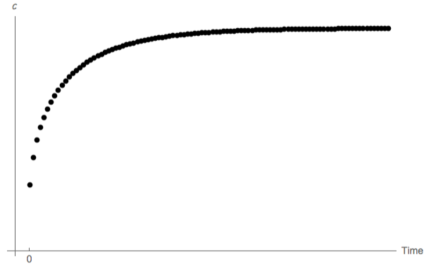
Figure 6 depicts the effect on the employed consumer’s spending by showing
each successive point in time as a dot. Starting at time 0 from the steady-state
level of consumption, the decrease in the future discounting rate (an increase in
patience) causes an instantaneous drop in the level of consumption. Starting from this
diminished base, consumption growth is subsequently faster than before the drop in
 .23
.23
Eventually consumption approaches its new, higher equilibrium ratio to permanent
income at a new, higher level of equilibrium  . This higher level of consumption is
financed in the long run by the higher interest income earned on the higher level of
wealth.
. This higher level of consumption is
financed in the long run by the higher interest income earned on the higher level of
wealth.
Note again, however, that equilibrium steady-state consumption growth is still equal to the
growth rate of income (this follows from the fact that there is a steady-state level for the ratio
of consumption to income,  ). This means that the higher level of wealth in equilibrium
ends up being precisely enough to reduce the precautionary term by an amount
that exactly offsets the fact that the
). This means that the higher level of wealth in equilibrium
ends up being precisely enough to reduce the precautionary term by an amount
that exactly offsets the fact that the  term in the Euler equation is now
smaller.
term in the Euler equation is now
smaller.
The final figures depict the time paths of consumption, market wealth, and the marginal
propensity to consume  following the decline in
  . These are implicit in the phase
diagram analysis, but the dots in these two new diagrams are spread out evenly over time
to give a sense of the time scale over which the model adjusts toward the steady
state.
. These are implicit in the phase
diagram analysis, but the dots in these two new diagrams are spread out evenly over time
to give a sense of the time scale over which the model adjusts toward the steady
state.
Loosely following Carroll and Jeanne (2009) (with some simplifications), this section extends
the model to analyze macroeconomic dynamics in a small open economy with a large number
of individuals, where the population statistics reflect the fulfillment of individual consumers’
ex ante expectations; for example, exactly proportion  of households who are
employed in period
of households who are
employed in period  become ‘unemployed’ before
  , so that the aggregate labor
supply of the ‘active’ (still employed) members of a generation evolves according
to
, so that the aggregate labor
supply of the ‘active’ (still employed) members of a generation evolves according
to
 | (43) |
where the first subscript denotes the date being examined and the second denotes the period of birth of the generation being examined.
We make strong assumptions that permit straightforward aggregation. The first such assumption is that newly unemployed households immediately migrate out of the country (think of British retirees moving to southern Spain).24 This means that macroeconomic variables will reflect only the circumstances of employed consumers, rather than a blend of the employed and the unemployed.
Each person is part of a single ‘generation’ of households born at the same time, and every
new generation is larger by the factor  than the newborn generation in the previous
period:
than the newborn generation in the previous
period:
 | (44) |
We assume that total production by the (surviving) members of a generation grows by the
factor  every period. If total production is to grow despite a shrinking number of surviving
members of the generation, production per active capita must grow by
every period. If total production is to grow despite a shrinking number of surviving
members of the generation, production per active capita must grow by  as per
(9).
as per
(9).
Consider the economy in some period 0 in which the size of the newborn population and the
wage rate have been normalized to  . If the economy has existed for
  periods (where
  is a negative number, indicating that the economy was created
before period 0), the ratio of the total population to the population of newborns will
be
is a negative number, indicating that the economy was created
before period 0), the ratio of the total population to the population of newborns will
be
 | (45) |
whose limit is a finite number so long as  , which we require.
Relative to the labor income of period 0’s newborn cohort ( ), the total labor
income in period 0 of the generation born in period
), the total labor
income in period 0 of the generation born in period  is
is  ; the sum of the incomes of
all of the two-period-old individuals is
; the sum of the incomes of
all of the two-period-old individuals is  , and so on; total labor income for all generations
in the economy in period 0 is
, and so on; total labor income for all generations
in the economy in period 0 is
 | (46) |
which is finite so long as either population growth is positive  (which we will assume)
or the economy has existed for a finite period of time (
(which we will assume)
or the economy has existed for a finite period of time ( ). In either case, the
proportion of aggregate income accounted for by a generation born at any specific
moment declines toward zero as time passes (old generations never die, they just fade
away).
). In either case, the
proportion of aggregate income accounted for by a generation born at any specific
moment declines toward zero as time passes (old generations never die, they just fade
away).
In the balanced growth equilibrium, the growth factor for aggregate population will
therefore be  and output per capita will increase by
  per period. Total labor income
therefore grows by
per period. Total labor income
therefore grows by 
We now examine this model under two assumptions about the initial ‘stake’ of newborns in the economy. (We use ‘stake’ to designate a transfer received by newborns). This is explicitly not an inheritance, as we have assumed that individuals have no bequest motive and newborns are unrelated to anyone in the existing population. Our motivation is to make the model more tractable, rather than to represent an important feature of the real world; we later perform simulations designed to show that the characteristics of the model with no ‘stake’ are qualitatively and quantitatively similar to those of the more tractable model with the ‘stake’ that makes the model tractable.
We first consider a version of the model in which an exogenous redistribution program guarantees that the behavior of employed households can be understood by analyzing the actions of a “representative employed agent.”
If a benevolent source outside the economy were to provide every newborn with an initial
transfer upon birth of size  , then the newborn’s total monetary resources would
be
, then the newborn’s total monetary resources would
be
 |
Thus, per-capita market resources for members of the newborn generation would be exactly equal to the target level of market resources for a person anticipating the future path of labor income that the members of the newborn generation actually anticipate (which is the same as the future path anticipated by all other generations as well).
If such a transfer policy had been in place forever, the economy at every point in time would
consist of employed households whose consumption had been equal to its steady-state value
 for their whole lives. That is, every individual agent in this economy would be identical in
their ratio of consumption, market resources, etc. to permanent labor income. The behavior of
any individual would therefore be fully captured by the behavior of a representative employed
agent.25
for their whole lives. That is, every individual agent in this economy would be identical in
their ratio of consumption, market resources, etc. to permanent labor income. The behavior of
any individual would therefore be fully captured by the behavior of a representative employed
agent.25
The foregoing scenario assumed that the ‘stake’ is provided by a mysterious ‘benevolent source outside the economy.’ Fortunately, there is an easy way to eliminate this problematic assumption: Assume that the stakes are financed by a wage tax.
The size of the required tax rate is calculated as follows. The total size of the resources transferred to the newborn generation must be
 | (47) |
where
 | (48) |
is the after-tax wage rate for the economy as a whole (and  is the steady state target ratio
of bank balances to after-tax wages).
is the steady state target ratio
of bank balances to after-tax wages).
From (46), the ratio of total aggregate labor income to the labor income of the newborn generation is
 | (49) |
so the aggregate wage tax rate required to finance a ‘stake’ of size  for newborns is given
by
for newborns is given
by
 | (50) |
Note, however, that in an economy where this tax has existed forever, the consequence
of the tax is effectively just a permanent reduction in after-tax labor income by
proportion  , compared to its value in the absence of the tax. Given the homotheticity of
the model, a permanent rescaling by a constant factor leaves the scaled version of
the individual’s problem (and its solution) unchanged. Thus we can conclude not
only that a representative agent exists in this economy, but that the steady-state
characteristics of the representative agent’s problem are identical (in ratio form) to the
characteristics of the unrescaled individual’s problem; that is,
, compared to its value in the absence of the tax. Given the homotheticity of
the model, a permanent rescaling by a constant factor leaves the scaled version of
the individual’s problem (and its solution) unchanged. Thus we can conclude not
only that a representative agent exists in this economy, but that the steady-state
characteristics of the representative agent’s problem are identical (in ratio form) to the
characteristics of the unrescaled individual’s problem; that is,  ,
,  , and so
on.
, and so
on.
Matters are not much more complicated outside the balanced growth steady state, so long
as we assume that the government always transfers the amount  to newborn households,
financed by the tax
to newborn households,
financed by the tax  derived above. Consider, for example, an economy that was in
steady-state equilibrium leading up to period
derived above. Consider, for example, an economy that was in
steady-state equilibrium leading up to period  , and at the beginning of
  there is a sudden
realization that future growth rates will be higher than those anticipated and experienced in
the past:
there is a sudden
realization that future growth rates will be higher than those anticipated and experienced in
the past:  after
after  . Since expected growth rates affect
  , the tax rate must be
immediately and permanently changed so that the generations born after
, the tax rate must be
immediately and permanently changed so that the generations born after  receive
a ‘stake’ of the proper new size. This change in
receive
a ‘stake’ of the proper new size. This change in  has two consequences for the
generations that survive from periods prior to
has two consequences for the
generations that survive from periods prior to  . Under the old tax rate, they would have
experienced
. Under the old tax rate, they would have
experienced  ; the change in expectations has no effect on
  or
or  but
changes the tax rate to
but
changes the tax rate to  . Thus these households will have an actual resource ratio
that differs from its new target value,
. Thus these households will have an actual resource ratio
that differs from its new target value,  , both because the after-tax income
scaling factor has changed and because the target ratio has changed from
, both because the after-tax income
scaling factor has changed and because the target ratio has changed from  to
to
 .
.
However, if we started out in steady-state, the ratio problem of every member of the continuing-employed population is identical to that of every other such household (though, again, their masses differ depending on age, etc); as a result, the dynamics of the economy are fully captured by keeping track of the relative weights in the economy of the (gradually diminishing) ‘representative shocked agent’ and the (gradually increasing) ‘representative new agent’ whose behavior is locked at its steady-state value.26
Figure 10 illustrates the dynamics in this economy using an experiment identical to one
explored above for the individual’s problem: In period 0 there is a one-off decline in the future
discounting rate (assuming the economy was in steady state before period 0). In the
previous model, each individual consumer’s consumption function shifted down, and
consumption experienced a discrete jump downward, because the agent became more
impatient. Here, there is a modest further effect: With more-patient consumers,
the tax rate that the government sets to finance a transfer of  to the newborns
must be larger (so that the ratio of initial assets to after-tax income is smaller).
Qualitatively, the dynamics are indistinguishable from the individual consumer’s dynamics
obtainable without working through the extra complication involved in accounting for the
‘stakes.’
to the newborns
must be larger (so that the ratio of initial assets to after-tax income is smaller).
Qualitatively, the dynamics are indistinguishable from the individual consumer’s dynamics
obtainable without working through the extra complication involved in accounting for the
‘stakes.’
The polar alternative to assuming that newborns get a ‘stake’ is to assume that newborns enter the economy with zero assets. Analysis of this version of the model must be performed using simulation methods, because households of different ages will have different levels of assets. (With a concave and nonanalytical consumption function, analytical aggregation cannot be performed.)
Our simulation procedure assumes that at date 0 the economy has existed
forever (so that the age distribution of relative populations and productivities are
at their steady-state values), but saving has been impossible prior to period
0.27
With everyone’s  , the ratio of market resources to permanent labor income is the same
for all individuals:
, the ratio of market resources to permanent labor income is the same
for all individuals:
 | (51) |
The consumption ratio in period 0 is therefore  for every household (regardless of age),
while the level of total labor income for a generation that is
for every household (regardless of age),
while the level of total labor income for a generation that is  periods old is
 .28
The population of such workers is
.28
The population of such workers is  , so aggregate consumption will be given by the
per-capita consumption ratio, multiplied by the per-capita level of permanent income,
multiplied by the population of workers still alive:
, so aggregate consumption will be given by the
per-capita consumption ratio, multiplied by the per-capita level of permanent income,
multiplied by the population of workers still alive:
 | (52) |
The longer a generation lives, the more time it will have had to save toward its target level of wealth; but newborns always begin life with no assets. After period 0, therefore, age-heterogeneity in assets and consumption ratios creeps into the population.
The foregoing discussion contains (in some cases implicitly) all the assumptions necessary to
conduct a simulation of this economy. Figure 11 shows the path of the ratio  starting from period 0 for an economy under our benchmark parameterization that generated
our earlier figures. The only extra parameter required beyond those used before is
starting from period 0 for an economy under our benchmark parameterization that generated
our earlier figures. The only extra parameter required beyond those used before is  ; we
choose
; we
choose  corresponding roughly to the postwar population growth rate in the United
States.
corresponding roughly to the postwar population growth rate in the United
States.
beginCDC
We consider now the consequences if the government creates a balanced-budget partial ‘unemployment insurance’ system. This system operates by imposing a labor income tax on the employed in order to finance transfers to the unemployed.29
Our definition of partial insurance starts by assuming that the ‘true’ labor income process is
the one specified above, but the government interferes with this process by selecting a
constant proportion  of the newly unemployed in each period who will be guaranteed
a ‘wage-indexed unemployment benefit’ that yields the same income they would
have received if they had not become unemployed. The lucky recipients of these
payments, however, are subject to a risk of termination from the unemployment
insurance program that matches the risk of becoming unemployed for the still-employed
consumers.
of the newly unemployed in each period who will be guaranteed
a ‘wage-indexed unemployment benefit’ that yields the same income they would
have received if they had not become unemployed. The lucky recipients of these
payments, however, are subject to a risk of termination from the unemployment
insurance program that matches the risk of becoming unemployed for the still-employed
consumers.
Under these circumstances, the household does not care whether it remains employed, or becomes unemployed but is selected for the unemployment insurance program: The dynamics of idiosyncratic future income are identical in the two cases.
Each generation finances its own unemployment insurance (this assumption is made to keep
the model as transparent as possible; it would not change things much to have the UI system
financed by the general government, but this would require some extra notation and
derivations, and discussion of essentially inconsequential intergenerational aspects of
unemployment insurance). The government sets the overall uninsurance rate  (‘uninsurance’
rather than ‘insurance’ rate because
(‘uninsurance’
rather than ‘insurance’ rate because  will be ‘no uninsurance’ or perfect insurance,
while
will be ‘no uninsurance’ or perfect insurance,
while  will be no insurance) and enforces exogenous taxation among the ‘truly
employed’ in the generation in such a way as to yield a modified ‘post-tax-and-transfer’
growth profile consistent with substituting
will be no insurance) and enforces exogenous taxation among the ‘truly
employed’ in the generation in such a way as to yield a modified ‘post-tax-and-transfer’
growth profile consistent with substituting  for
for  in the derivations above,
where
in the derivations above,
where
 | (53) |
and  guarantees that the insurance program results in a reduction of idiosyncratic
income risk.
guarantees that the insurance program results in a reduction of idiosyncratic
income risk.
Substituting  for
for  in the prior derivations, this scheme is consistent with the
generational budget constraint because, as noted above, the individual income growth process
was constructed so that the present discounted value of income remains invariant to the size of
in the prior derivations, this scheme is consistent with the
generational budget constraint because, as noted above, the individual income growth process
was constructed so that the present discounted value of income remains invariant to the size of
 , and the aggregate income of a generation grows by
  regardless of the underlying
idiosyncratic unemployment risk.
regardless of the underlying
idiosyncratic unemployment risk.
This scheme is attractive because in practice it simply requires solving the model specified
above for a different value of  . This will make solution and simulation of the model
particularly simple.
. This will make solution and simulation of the model
particularly simple.
In addition to the consumption function, the solution procedure
produces an estimate of the representative employed agent’s value
function.30
Value depends on current resources, but also (numerically) on all of the parameters in the
calibration of the model. We are particularly interested in how value relates to expected labor
productivity growth  , to the ‘true’ unemployment risk
  , and to the generosity of the
unemployment insurance program
, and to the generosity of the
unemployment insurance program  . Writing
 | (54) |
(where we separate the state variable  from the parameters using a semicolon) we can
investigate a variety of interesting questions. Some examples:
from the parameters using a semicolon) we can
investigate a variety of interesting questions. Some examples:
 such that
 | (55) |
 . The cost is increased unemployment risk
  . For a given generosity of
unemployment insurance, how much extra growth is necessary to offset the utility cost
of greater risk? That is, supposing the relationship between
. For a given generosity of
unemployment insurance, how much extra growth is necessary to offset the utility cost
of greater risk? That is, supposing the relationship between  and
and  is
indexed by a parameter
is
indexed by a parameter  , e.g.
  , what is the
  for
which
for
which
 | (56) |
 ?
?Many more such questions can be imagined. endCDC
Using from MathFacts the second-order and then the first-order Taylor approximations
![[TaylorTwo ]](TractableBufferStock431x.svg)
 and then
 ![[TaylorOne ]](TractableBufferStock433x.svg)
 ,
the expression in braces in (11) can be rewritten
,
the expression in braces in (11) can be rewritten
![{ [( ce )ρ ]}1 ∕ρ { [( cu + ce − cu ) ρ ]}1∕ρ
1 + ℧ -t+u1- − 1 = 1 + ℧ -t+1----t+u1----t+1 − 1
ct+1 ct+1
= {1 + ℧ [(1 + ∇ )ρ − 1]}1∕ρ
{ [ t+1 ]}
≈ 1 + ℧ 1 + ρ∇t+1 + ρ(∇t+1 )2ω − 1 1∕ρ
{ }1∕ρ
= 1 + ρ℧ (∇t+1 + (∇t+1)2ω )
≈ 1 + ℧ (1 + ∇ ω) ∇ ,
t+1 t+1](TractableBufferStock435x.svg) |
which leads directly to (17) in the main text.
At a steady-state value of  , both
  and
and  hold (equations (29) and (31));
for convenience defining
hold (equations (29) and (31));
for convenience defining  ,
,
 | (57) |
But since  is a positive number, at
  the
the  locus’s
value is
locus’s
value is  while the value of the
  locus is zero, the two loci
can intersect for a positive
locus is zero, the two loci
can intersect for a positive  only if the slope of the
  locus is
greater:31
locus is
greater:31
 | (58) |
which is equivalent to
 | (59) |
where the LHS is (proportional to) the slope of  and the RHS is (proportional to) the
slope of
and the RHS is (proportional to) the
slope of  . beginCDC
It is not totally obvious why these are equivalent, so here’s the derivation.
 | (60) |
endCDC
For any fixed  and
and  and
and  we can find some
  for which
  , and
using this
, and
using this  it turns out to be useful to rewrite
 | (61) |
Note for future use that (61) implies that whenever  , the FHWC
 fails (‘human
wealth is infinite’) because
fails (‘human
wealth is infinite’) because  .
.
Multiplying both sides of (59) by  then substituting the expression for
  from (61) gives
 | (62) |
Since  and
and  (as guaranteed by the RIC), (62) is satisfied whenever the
FHWC
(as guaranteed by the RIC), (62) is satisfied whenever the
FHWC fails (
 ) and
) and  . We now show that under these conditions,
 .
.
 from (19) is:
 | (63) |
but note that
 | (64) |
and in the case where  ,
,  must also be 1, implying that
  (the
RIC) so that
(the
RIC) so that  and so
  and hence
  . The other interesting case is
when
. The other interesting case is
when  so that
  and
and  . In this case
 and so
  and so
  is even more positive so that
  is even more
strongly
is even more
strongly  . Similar logic holds for any
  .
.
Thus, we can conclude that, when human wealth is infinite (that is, if  ), a target
 will exist.
In the case where human wealth is finite ( ), we need the RHS of (62) not merely to be
positive, but to exceed a specific positive number,
), we need the RHS of (62) not merely to be
positive, but to exceed a specific positive number,  :
:
![1∕ρ
κ(1 + ϖ ) > ((α − 1 )℧ ∕(1) − ℧ )
1∕ρ (α − 1)℧
(1 + ϖ ) > ---------
( κ (1 − ℧ )) ρ
(α-−-1)℧-
(1 + ϖ) > κ (1 − ℧ )
( ) ρ
(ÞÞÞ −ρ− 1)℧−1 = ϖ > (α-−-1)℧- − 1
ΦΦΦ κ (1 − ℧ )
[ ((α − 1)℧) ρ ]
(ÞÞÞ−ΦΦΦ ρ− 1) > ℧ --------- − 1
κ(1 − ℧)
−ρ [( (α − 1 )℧ ) ρ ]
ÞÞÞΦΦΦ > 1 + ℧ --------- − 1
( κ (1 − ℧ ) )
| | −1∕ρ
||{ [( ) ρ ]||}
ÞÞÞ < 1 + ℧ (α-−-1-)℧- − 1
ΦΦΦ || κ (1 − ℧) ||
|( ◟--------◝◜--------◞|)
≡χ](TractableBufferStock495x.svg) | (65) |
and the boundary will be the point at which this expression holds with equality.
An increase in impatience caused by an increase in the pure time preference rate  (equivalently, a reduction in
  ) has the effect of reducing growth-patience (the LHS of (65))
and of increasing the RHS. This means that there will be some time preference rate sufficiently
large (some
) has the effect of reducing growth-patience (the LHS of (65))
and of increasing the RHS. This means that there will be some time preference rate sufficiently
large (some  sufficiently small) to guarantee that the condition holds with equality. Then
(65) will always be satisfied by any
sufficiently small) to guarantee that the condition holds with equality. Then
(65) will always be satisfied by any  satisfying
 | (66) |
beginCDC
![=R∕ΦΦΦ
◜(---◞◟---)◝ { [( ) ρ ]} −1∕ρ
1-−-℧--- (α-−-1)℧-
ÞÞÞR 1 − α℧ = ÞÞÞΦΦΦ = 1 + ℧ κ (1 − ℧ ) − 1](TractableBufferStock501x.svg) |
and note that if we reduce  incrementally the denominator on the LHS increases so the
LHS decreases, while the RHS increases. Under the new value of
incrementally the denominator on the LHS increases so the
LHS decreases, while the RHS increases. Under the new value of  , therefore,
  , if the
condition held with equality before it now holds with inequality.
, if the
condition held with equality before it now holds with inequality.
endCDC
Since we have assumed the RIC (so that  ), as
), as  or
or  , (65) asymptotes to
the GIC
, (65) asymptotes to
the GIC for any given value of
  .
.
The apparently harder case is when  and
and  . But note that we will have found
 if we can find the corresponding
  at which the first term in
  reaches
1:
reaches
1:
![( )
(α − 1)℧ ρ
---------------- = 1
((1 − ÞÞÞR )(1 − ℧ ) )
---(α-−--1)℧----
(1 − ÞÞÞR)(1 − ℧ ) = 1
( )
(α-−-1)℧- = 1 − ÞÞÞ
(1 − ℧ ) R
( (α − 1)℧ )
1 − --------- = ÞÞÞR
[ ( (1 − ℧ ))]
(α − 1)℧ 1∕ρ
1 − --------- = (R β) ∕R
[ ( (1 − ℧ ))] ρ
ρ (α-−-1)℧-
R 1 − (1 − ℧ ) = (R β)
[ ( )] ρ
Rρ−1 1 − (α-−-1)℧- = ¯βFHW.
(1 − ℧ )](TractableBufferStock515x.svg) | (67) |
Somewhat miraculously, at this value of  , because
  , (65) holds with equality, which
means that
, (65) holds with equality, which
means that  . This means that the GIC
 defines the definitive boundary
condition: A finite target
defines the definitive boundary
condition: A finite target  exists so long as
We have just demonstrated that satisfying the GIC condition is necessary and sufficient
to guarantee existence of a target
condition is necessary and sufficient
to guarantee existence of a target  . But we suggested earlier that a weaker
condition, the GIC-TBS, guarantees the existence of a well-defined consumption
function.
. But we suggested earlier that a weaker
condition, the GIC-TBS, guarantees the existence of a well-defined consumption
function.
This can be understood as follows. Rewrite the requirement for existence of a target, (59), as
 | (68) |
or taking logs we have approximately
 | (69) |
The LHS captures the slope of the  locus, which is
  modified
by
modified
by  whose difference from
  captures the degree of growth
(im)patience.32
The RHS captures the slope of the
captures the degree of growth
(im)patience.32
The RHS captures the slope of the  locus. Recall that the inequality captures the
fact that a target
locus. Recall that the inequality captures the
fact that a target  exists if these two loci intercept, which happens if the slope of
 exceeds that of
  .
.
If the consumer is ‘growth patience poised’ (that is,  ), then
  and the slope
of the
and the slope
of the  locus is identical to the
  that characterizes the perfect foresight
consumption function. In this case (69) becomes
that characterizes the perfect foresight
consumption function. In this case (69) becomes
 | (70) |
which is the (log version of) the GIC . The condition cannot hold both as an equality
 (our starting assumption) and an inequality
  (the conclusion of (70)).
This contradiction constitutes a proof that exactly at
(the conclusion of (70)).
This contradiction constitutes a proof that exactly at  a target does not
exist.
a target does not
exist.
As noted above, if the consumer is growth-impatient ( ) then
  and the slope
of
and the slope
of  is monotonically increased as the degree of growth-impatience increases (so that
target
is monotonically increased as the degree of growth-impatience increases (so that
target  is diminished).
But if the consumer is growth-patient ( ) then
  and the slope of
  is diminished
(which reflects the fact that the greater the degree of patience, the lower will consumption be for any
given
is diminished
(which reflects the fact that the greater the degree of patience, the lower will consumption be for any
given  ).33
The lower bound is defined by the point at which the degree of growth patience becomes so
strong that the slope of
).33
The lower bound is defined by the point at which the degree of growth patience becomes so
strong that the slope of  reaches zero (when
  ; equivalently,
  reaches -1).
This restricts the permissible degree of growth patience, because
reaches -1).
This restricts the permissible degree of growth patience, because  requires (rewrite
(12)):
requires (rewrite
(12)):
 | (71) |
Expanding on a discussion in the main text, the numerator in the leftmost expression
reflects the sense in which the unemployment risk acts in a manner similar to the effect
of an extra degree of discounting (reflecting the fact that the relevant condition
applies only so long as the consumer remains in employment – a condition whose
probability is  ), while the denominator reflects the mechanical effect in which the
relevant measure of growth is boosted by the adjustment that preserves human
wealth. Writing the perfect foresight version of the growth patience factor as
), while the denominator reflects the mechanical effect in which the
relevant measure of growth is boosted by the adjustment that preserves human
wealth. Writing the perfect foresight version of the growth patience factor as  (which is just the limit as
  ), we can see that the expression on the LHS is just
 which is smaller than
  because
  and
and  . So, the
GIC-TBS holds whenever the plain-vanilla GIC
. So, the
GIC-TBS holds whenever the plain-vanilla GIC holds, but not vice-versa; there
are parametric configurations in which a perfect-foresight consumer with income
growth rate
holds, but not vice-versa; there
are parametric configurations in which a perfect-foresight consumer with income
growth rate  would not satisfy the relevant GIC
 (so, their wealth-to-income
ratio would go to infinity), but the same consumer faced the same human wealth
but with an unemployment risk
(so, their wealth-to-income
ratio would go to infinity), but the same consumer faced the same human wealth
but with an unemployment risk  would have a finite target wealth-to-income
ratio.
would have a finite target wealth-to-income
ratio.
The easiest way to understand all of this is graphically. A notebook Carroll (Ongoing) (see
references for details) in the code archive associated with these lecture notes shows how this
works for alternative values of 

To simplify the expressions in the derivations below, we define  so
that
so
that  and we drop the
  superscripts, allowing (29) to be rewritten
as
superscripts, allowing (29) to be rewritten
as
 | (72) |
If a target value  exists it will be at the point of intersection between the
  and
the
and
the  loci:
loci:
 | (73) |
A first point about this formula is suggested by the fact that
 | (74) |
which is likely to increase as  approaches
zero.34
Note that the limit as
approaches
zero.34
Note that the limit as  is infinity, which implies that
  . This is precisely
what would be expected from this model in which consumers are impatient but
self-constrained to have
. This is precisely
what would be expected from this model in which consumers are impatient but
self-constrained to have  : As the risk gets infinitesimally small, the amount by which
target
: As the risk gets infinitesimally small, the amount by which
target  exceeds its minimum possible value shrinks to zero.
We now show that the RIC and GIC ensure that the denominator of the fraction in (73)
is positive:
ensure that the denominator of the fraction in (73)
is positive:
 |
However, note that  also affects
  ; thus, the first inequality above does not necessarily
imply that the denominator is decreasing as
; thus, the first inequality above does not necessarily
imply that the denominator is decreasing as  moves from
  to
to  .
.

Now defining
 | (75) |
under certain conditions we can obtain further insight into (73) using
a judicious mix of first- and second-order Taylor expansions (along with
 ):35
):35
 | (76) |
But
 | (77) |
which is guaranteed to be positive by the GIC , but which can take any value in the interval
 . Note, however, that the approximations above are valid only if
  is ‘small’ which
requires that the degree of growth impatience be small relative to the size of the
unemployment risk. Thus, the formulae derived above (and used below) are reliable only in
rather special circumstances, in particular when the consumer is only very slightly
growth-impatient.36
Under these circumstances, this approximation can be substituted into (76) to obtain
is ‘small’ which
requires that the degree of growth impatience be small relative to the size of the
unemployment risk. Thus, the formulae derived above (and used below) are reliable only in
rather special circumstances, in particular when the consumer is only very slightly
growth-impatient.36
Under these circumstances, this approximation can be substituted into (76) to obtain
 | (78) |
and inspired by Kimball (1990) defining a term related to the excess of prudence over the logarithmic case,
 | (79) |
(73) can be approximated by
 | (80) |
where negative signs have been preserved in front of the  and
and  terms as a
reminder that the GIC
terms as a
reminder that the GIC and the RIC imply these terms are themselves negative
(so that
and the RIC imply these terms are themselves negative
(so that  and
and  are positive). Ceteris paribus, an increase in relative
risk aversion
are positive). Ceteris paribus, an increase in relative
risk aversion  will increase
  and thereby decrease the denominator of (80).
This suggests that greater risk aversion will result in a larger target level of
wealth.37
and thereby decrease the denominator of (80).
This suggests that greater risk aversion will result in a larger target level of
wealth.37
The formula also provides insight about how the human wealth effect works in equilibrium.
All else equal, the human wealth effect is captured by the  term in the denominator of
(80), and it is obvious that a larger value of
term in the denominator of
(80), and it is obvious that a larger value of  will result in a smaller target value for
 . But it is also clear that the size of the human wealth effect will depend on the
magnitude of the patience and prudence contributions to the denominator, and that
those terms can easily dominate the human wealth effect. This reduction in the
human wealth effect is interesting because practitioners have known at least since
Summers (1981) that the human wealth effect is implausibly large in the perfect foresight
model.
. But it is also clear that the size of the human wealth effect will depend on the
magnitude of the patience and prudence contributions to the denominator, and that
those terms can easily dominate the human wealth effect. This reduction in the
human wealth effect is interesting because practitioners have known at least since
Summers (1981) that the human wealth effect is implausibly large in the perfect foresight
model.
For (80) to make sense, we need the denominator of the fraction to be a positive number; defining
 | (81) |
this means that we need:
 | (82) |
But since the RIC guarantees  and the GIC
 guarantees
 (which, in turn, guarantees
  ), this condition must
hold.38
), this condition must
hold.38
The same set of derivations imply that we can replace the denominator in (80) with the negative of the RHS of (82), yielding a more compact expression for the target level of resources,
 | (83) |
This formula makes plain the fact that an increase in either form of impatience, by increasing the denominator of the fraction in (83), will reduce the target level of assets.
We are now in position to discuss (80), understanding that the impatience conditions guarantee that its denominator is a positive number.
Two specializations of the formula are particularly useful. The first is the case where  (logarithmic utility). In this case
 | (84) |
and the approximation becomes
 | (85) |
which neatly captures the effect of an increase in human wealth (via either increased  or
reduced
or
reduced  ), the effect of increased impatience
  , or the effect of a reduction in
unemployment risk
, or the effect of a reduction in
unemployment risk  in reducing target wealth.
The other useful case to consider is where  but
but  . In this case, we
have
. In this case, we
have
 | (86) |
so that
 | (87) |
where the additional term involving  in this equation captures the fact that an increase in
the prudence term
in this equation captures the fact that an increase in
the prudence term  shrinks the denominator and thereby boosts the target level of
wealth.39
shrinks the denominator and thereby boosts the target level of
wealth.39
To solve the model by the method of reverse
shooting,40
we need  as a function of
  . Starting with (11):
![( ce ) { [( ce ) ρ ]}1 ∕ρ
-t+1e- = ΦΦΦ −1(Rβ )1∕ρ 1 + ℧ -tu+1 − 1
ct ct+1
( )
e | cet+1 |
ct = ( -----------{------[(----e----)-ρ---]-}1∕ρ)
ΦΦΦ−1(R β)1∕ρ 1 + ℧ κ(cmte+1−-1)- − 1
{ [( t+1 ) ]}
−1∕ρ e cet+1 ρ − 1∕ρ
= ΦΦΦ (Rβ ) ct+1 1 + ℧ ----e------- − 1 .
κ(m t+1 − 1)](TractableBufferStock648x.svg) | (88) |
Inverting (30), the reverse shooting equation for  is
is
 | (89) |
The reverse shooting approximation will be more accurate if we use it to obtain estimates of
the marginal propensity to consume as well. These are obtained by differentiating the
consumption Euler equation with respect to  :
:
![ℶ
◜----◞◟-----◝
u′(ce(mt )) = RN rm βΦΦΦ1− ρ𝔼t[u′(c∙(mt+1 ))]
u′′(ce(m ))κκκe(m ) = ℶRN rm (1 − κκκe(m )) 𝔼 [u ′′(c∙(m ))κκκ∙(m )]
t t t t t+1 t+1](TractableBufferStock652x.svg) | (90) |
so that defining, e.g.,  we have
![e e ′′ e [ ′′ ∙ ∙ ]
κt = (1 − κt) ℶ◟RN--rm-(1∕u-(ct)◝)◜𝔼t-u--(ct+1)κt+1◞
≡♮t+1
e
(1 + ♮t+1)κt = ♮t+1
( ♮t+1 )
κet = -------- .
1 + ♮t+1](TractableBufferStock654x.svg) |
At the target level of  we have
![♮∕RNrm ℶ =1
◜ ---′′--e-◞◟ --′′-∙--◝∙ ◜-′′-e-◞◟-′′-e-◝ e ′′ u ′′ e
(1∕u (ˆc )) 𝔼t[u (c )κ ] = //℧ (u (cˆ)∕u (ˆc ))κ + ℧ (u (ˆc )∕u (ˆc ))κ](TractableBufferStock656x.svg) |
so that
 | (91) |
yielding from (91) a quadratic equation in  :
:
 | (92) |
which has one solution for  in the interval
 ![[0,1]](TractableBufferStock661x.svg) , which is the MPC at target
wealth.41
, which is the MPC at target
wealth.41
The limiting MPC as consumption approaches zero,  will also be useful; this is obtained
by noting that utility in the employed state next year becomes asymptotically irrelevant as
will also be useful; this is obtained
by noting that utility in the employed state next year becomes asymptotically irrelevant as
 approaches zero, so that
 |
so that from (91) we have
 | (93) |
which implicitly defines  . An explicit solution is not available, but after parameter
values have been defined a numerical rootfinder can calculate a solution almost
instantly.
. An explicit solution is not available, but after parameter
values have been defined a numerical rootfinder can calculate a solution almost
instantly.
Finally, it will be useful to have an estimate of the curvature (second derivative) of the
consumption function. This can be obtained by a procedure analogous to the one used to
obtain the MPC: differentiate the differentiated Euler equation (90) again. Noting that
 we can obtain:
![(κκκe)2u′′′(ce) + κκκe′u′′(ce) =
t t{ et′ t′′ ∙ ∙ e 2( ∙ 2 ′′′ ∙ ′′ e e′ )}
ℶRN rm (− κκκt )𝔼t [u (ct+1)κκκt+1] + RN rm (1 − κκκt) 𝔼t[(κκκt+1) u (ct+1)] + //℧u (ct+1)κκκt+1](TractableBufferStock668x.svg) |
so that
![( 2 e 2( ∙ 2 ′′′ ∙ ′′ e e′ ) e 2 ′′′ e )
κκκe′ = ℶRN--rm--(1-−-κκκt)--𝔼t-[(κκκt+1)-u--(ct+1)] +-//℧u-(ct+1)κκκt+1-−--(κκκ-t)u--(ct)
t u′′(cet) + ℶRN rm 𝔼t [u′′(c∙t+1)κκκ∙t+1]](TractableBufferStock669x.svg) |
which can be further simplified at the target because  so
that
so
that
![( 2 e 2 ∙ 2 ′′′ ∙ e 2 ′′′ e )
κe′ = ------ℶRN--rm--(1 −-κ-)-𝔼t[(κ-)-u-(c-)] −-(κ-)-u-(ˆc)----- .
u ′′(ˆce) + ℶRN rm 𝔼t[u′′(c∙)κ ∙] − ℶRN rm2 (1 − κe)2//℧u ′′(ˆce)](TractableBufferStock671x.svg) | (94) |
Another differentiation of (94) similarly allows the construction of a formula for the value of
 at the target
  ; in principle, any number of derivatives can be constructed in this
manner.42
; in principle, any number of derivatives can be constructed in this
manner.42
beginCDC
 approaches infinity, the ratio
 approaches a constant
  . If we make such an assumption, then we can use other
results to show that
. If we make such an assumption, then we can use other
results to show that
 | (95) |
endCDC
beginCDC
 will be dominated by the outcomes for the
unemployed consumer so that
will be dominated by the outcomes for the
unemployed consumer so that
 |
becomes
 | (96) |
which approaches a function  as
as  approaches zero. This is inconvenient, because an
infinite second derivative cannot be used for a data point in the set of interpolating points.
endCDC
approaches zero. This is inconvenient, because an
infinite second derivative cannot be used for a data point in the set of interpolating points.
endCDC
Reverse shooting requires us to solve separately for an approximation to the consumption
function above the steady state and another approximation below the steady state. Using the
approximate steady-state  and
and  obtained above, we begin by picking a very small
number for
obtained above, we begin by picking a very small
number for  and then creating a Taylor approximation to the consumption function near
the steady state:
and then creating a Taylor approximation to the consumption function near
the steady state:
 |
and then iterate the reverse-shooting equations until we reach some period  in which
  escapes some pre-specified interval
 ![[me, ¯me ]](TractableBufferStock689x.svg) (where the natural value for
(where the natural value for  is 1 because
this is the
is 1 because
this is the  that would be owned by a consumer who had saved nothing in the prior period
and therefore is below any feasible value of
that would be owned by a consumer who had saved nothing in the prior period
and therefore is below any feasible value of  that could be realized by an optimizing
consumer). This generates a sequence of points all of which are on the consumption function.
A parallel procedure (substituting
that could be realized by an optimizing
consumer). This generates a sequence of points all of which are on the consumption function.
A parallel procedure (substituting  for
for  in (97) and where appropriate in the
corresponding equation for
in (97) and where appropriate in the
corresponding equation for  generates the sequence of points for the approximation below
the steady state. Taken together with the already-derived characterization of the
function at the target level of wealth, these points constitute the basis for a piecewise
second-order interpolating approximation to the consumption function on the interval
generates the sequence of points for the approximation below
the steady state. Taken together with the already-derived characterization of the
function at the target level of wealth, these points constitute the basis for a piecewise
second-order interpolating approximation to the consumption function on the interval
![e e
[m- , ¯m ]](TractableBufferStock696x.svg) .
.
As a preliminary, note that since  , value for an unemployed consumer
is
, value for an unemployed consumer
is
 | (97) |
where the RIC guarantees that the denominator in the fraction is a positive number.
From this we can see that value for the normalized problem is similarly:
 | (98) |
Turning to the problem of the employed consumer, we have
![e e 1−ρ ∙
v (mt) = u (ct) + βΦΦΦ 𝔼t[v (mt+1 )]](TractableBufferStock700x.svg) | (99) |
and at the target level of market resources this will be unchanging for a consumer who remains employed so that
 | (100) |
Given these facts, our recursion for generating a sequence of points on the consumption function can be used at the same time to generate corresponding points on the value function from
 | (101) |
with the first iteration point generated by numerical integration from
 | (102) |
beginCDC
 | (103) |
which leads to an approximation of the level of value at  using
using
 |
endCDC
With the above results in hand, the model is solved and the various functions constructed as
follows. Define  as a vector of points that characterizes a particular
situation that an optimizing employed household might be in at any given point in time. Using
the backwards-shooting functions derived above, for any point
as a vector of points that characterizes a particular
situation that an optimizing employed household might be in at any given point in time. Using
the backwards-shooting functions derived above, for any point  we can construct the
sequence of points that must have led up to it:
we can construct the
sequence of points that must have led up to it:  and
and  and so on. And using the
approximations near the steady state like (97), we can construct a vector-valued function
and so on. And using the
approximations near the steady state like (97), we can construct a vector-valued function
 that generates, e.g.,
  .
.
Now define an operator  as follows:
  applied to some starting point
  uses the
backwards dynamic equations defined above to produce a vector of points
uses the
backwards dynamic equations defined above to produce a vector of points  consistent with the model until the
  that is produced goes outside of the pre-defined
bounds for solving the problem.
that is produced goes outside of the pre-defined
bounds for solving the problem.
We can merge the points below the steady state with the steady state with the points above
the steady state to produce  . These points can then be used
to generate appropriate interpolating approximations to the consumption function and other
desired functions.
. These points can then be used
to generate appropriate interpolating approximations to the consumption function and other
desired functions.
Designate, e.g., the vector of points on the consumption function generated in this manner
by ![...
⋆[c]](TractableBufferStock719x.svg) , so that
, so that
![( m [1] {c [1],κe[1],κe′[1]} )
| e e′ |
{...⋆[m ],{..⋆.[c],.⋆..[κe],...⋆[κe′]}⊺}⊺ = | m [2] {c [2],κ [2],κ [2]} |
( ... ... )
m [N ] {c[N ],κe [N ],κe′[N ]}](TractableBufferStock720x.svg) | (104) |
where  is the number of points that have been generated by the merger of the backward
shooting points described above.
is the number of points that have been generated by the merger of the backward
shooting points described above.
The object (104) is not an arbitrary example; it reflects a set of values that uniquely define a fourth order piecewise polynomial spline such that at every point in the set the polynomial matches the level and first derivative included in the list. Standard numerical mathematics software can produce the interpolating function with this input; for example, the syntax in Mathematica is simply
![... ... ... e ... e′ ⊺ ⊺
cE = Interpolation [{⋆ [m ],{⋆[c],⋆[κ ],⋆[κ ]} } ].](TractableBufferStock722x.svg) | (105) |
which creates a function  that is a
  interpolating polynomial connecting these
points.
interpolating polynomial connecting these
points.
beginCDC
![[0, ¯me ]](TractableBufferStock725x.svg) .43
This approximation, however, becomes highly problematic when evaluated outside of this
range. (Polynomial interpolations tend to ‘blow up’ when extended outside the interval on
which they are constructed.)
.43
This approximation, however, becomes highly problematic when evaluated outside of this
range. (Polynomial interpolations tend to ‘blow up’ when extended outside the interval on
which they are constructed.)
endCDC
The reverse shooting algorithm terminates at some finite maximum point
 , but for completeness it is useful to have an approximation to the
consumption function that is reasonably well behaved for any
, but for completeness it is useful to have an approximation to the
consumption function that is reasonably well behaved for any  no matter how
large.44
no matter how
large.44
Since we know that the consumption function in the presence of uncertainty asymptotes to the perfect foresight function, we adopt the following approach. Defining the level of precautionary saving as45
 | (106) |
we know (see the discussion below in appendix section G) that
 | (107) |
Defining  , a convenient functional form to postulate for the propensity to
precautionary-save is
, a convenient functional form to postulate for the propensity to
precautionary-save is
 | (108) |
with derivatives
 | (109) |
Evaluated at  (for which
  and its derivatives will have numerical values assigned by
the reverse-shooting solution method described above), this is a system of four equations in
four unknowns and, though nonlinear, can be easily solved for values of the
and its derivatives will have numerical values assigned by
the reverse-shooting solution method described above), this is a system of four equations in
four unknowns and, though nonlinear, can be easily solved for values of the  and
and  coefficients that match the level and first three derivatives of the “true”
  function.46
beginCDC
 , we define
 | (110) |
which has many useful properties, among them that as  ,
,  . The values of
 can be computed at the same points for which values of
  and its derivatives
were constructed using the reverse-shooting method. Outside of the interval, we can use the
consumption function to produce
and its derivatives
were constructed using the reverse-shooting method. Outside of the interval, we can use the
consumption function to produce  by numerical integration from the boundaries of the
interval.
by numerical integration from the boundaries of the
interval.
To complete this scheme, we will need the derivatives:
 | (111) |
along with the limits:
![lim n(m ) = 0
m→0
′ e −ρ 1−/ρ
mlim→0 n(m ) = lmim→0(¯κ m ) (/ρv) /ρ
e −ρ e 1−ρ ∙ -ρ-
= lmim→0(¯κ m ) (/ρ(u(¯κ m ) + βΦΦΦ 𝔼t[vt+1]))1−ρ
e −ρ e 1−ρ u e -ρ-
= lmim→0(¯κ m ) (/ρ(u(¯κ m ) + βΦΦΦ ℧v t+1(m (1 − ¯κ ))))1− ρ
e −ρ e 1−ρ e e -ρ-
= lim (¯κ m ) (/ρ(u(¯κ m ) + βΦΦΦ ℧u (m (1 − ¯κ )¯κ )𝔳))1−ρ
m →0 -ρ-
= lim (¯κem )−ρ((¯κem )1∕(1−ρ)(1 + β ΦΦΦ1−ρ℧ (1 − ¯κe)1−ρ𝔳))1−ρ
m →0 -ρ-
= lim (1 + βΦΦΦ1 −ρ℧(1 − ¯κe)1−ρ𝔳)1−ρ
m →0](TractableBufferStock749x.svg) | (112) |
Carroll (2022) shows that the value function can be bounded for  by a function of
the form
by a function of
the form
 | (113) |
for any  .
.
Thus, dropping arguments we define
 | (114) |
Thus, dropping arguments we define
 | (115) |
and  must be computed by application of L’Hopital’s rule from
 | (116) |
and
 | (117) |
 | (118) |
Finally, the limit as  goes to zero will be useful:
 | (119) |
Another solution is to note that value for this problem is bounded below by the value that would be experienced by an unemployed consumer and above by the value that would be experienced by a consumer with the same PDV of income but whose income was perfectly certain,
 | (120) |
so that for any  value can be represented by
 | (121) |
Since  and
and  are analytical functions, this means that our problem is effectively
reduced to approximating the function
are analytical functions, this means that our problem is effectively
reduced to approximating the function  whose value is bounded in the
 ![[0,1]](TractableBufferStock767x.svg) interval.
interval.
endCDC

The text asserts that if  the consumption function for a finite-horizon employed
consumer approaches the
the consumption function for a finite-horizon employed
consumer approaches the  function that is optimal for a perfect-foresight consumer with
the same horizon,
function that is optimal for a perfect-foresight consumer with
the same horizon,
 | (122) |
This proposition can be proven by careful analysis of the consumption Euler equation,
noting that as  approaches infinity the proportion of consumption will be financed out of
(uncertain) labor income approaches zero, and that the magnitude of the precautionary effect
is proportional to the square of the proportion of such consumption financed out of uncertain
labor income.
approaches infinity the proportion of consumption will be financed out of
(uncertain) labor income approaches zero, and that the magnitude of the precautionary effect
is proportional to the square of the proportion of such consumption financed out of uncertain
labor income.
A footnote also claims that for employed consumers,  approaches a different,
but still well-defined, limit even if
approaches a different,
but still well-defined, limit even if  , so long as the impatience condition
holds.
, so long as the impatience condition
holds.
It turns out that the limit in question is the one defined by the solution to a perfect foresight problem with liquidity constraints. A semi-analytical solution does exist in this case, but it requires formidable notation and analysis to present and understand, so the details are not presented here. A continuous-time treatement can be found in Park (2006).
Blanchard, Olivier J. (1985): “Debt, Deficits, and Finite Horizons,” Journal of Political Economy, 93(2), 223–247.
Carroll, Christopher (2020): “Theoretical Foundations of Buffer Stock Saving,” Econ-ARK REMARK, Available at https://econ-ark.github.io/BufferStockTheory.
Carroll, Christopher D. (1992): “The Buffer-Stock Theory of Saving: Some Macroeconomic Evidence,” Brookings Papers on Economic Activity, 1992(2), 61–156, https://www.econ2.jhu.edu/people/ccarroll/BufferStockBPEA.pdf.
__________ (1997): “Buffer Stock Saving and the Life Cycle/Permanent Income Hypothesis,” Quarterly Journal of Economics, CXII(1), 1–56.
__________ (2001): “Death to the Log-Linearized Consumption Euler Equation! (And Very Poor Health to the Second-Order Approximation),” Advances in Macroeconomics, 1(1), Article 6, https://www.econ2.jhu.edu/people/ccarroll/death.pdf.
__________ (2022): “Theoretical Foundations of Buffer Stock Saving,” Submitted.
__________ (Ongoing): “Mathematica Notebook Illustrating Target Wealth In Cases Where FHWC-TBS Fails,” ./Code/Mathematica/Examples/ManipulateParameters/When-FHWC-Holds.nb, Download archive and open Mathematica notebook.
Carroll, Christopher D., and Olivier Jeanne (2009): “A Tractable Model of Precautionary Reserves, Net Foreign Assets, or Sovereign Wealth Funds,” NBER Working Paper Number 15228, https://www.econ2.jhu.edu/people/ccarroll/papers/cjSOE.
Carroll, Christopher D., and Miles S. Kimball (1996): “On the Concavity of the Consumption Function,” Econometrica, 64(4), 981–992, https://www.econ2.jhu.edu/people/ccarroll/concavity.pdf.
Carroll, Christopher D., and Miles S. Kimball (2007): “Precautionary Saving and Precautionary Wealth,” Palgrave Dictionary of Economics and Finance, 2nd Ed., https://www.econ2.jhu.edu/people/ccarroll/papers/PalgravePrecautionary.pdf.
Friedman, Milton A. (1957): A Theory of the Consumption Function. Princeton University Press.
Hall, Robert E. (1988): “Intertemporal Substitution in Consumption,” Journal of Political Economy, XCVI, 339–357, Available at http://www.stanford.edu/~rehall/Intertemporal-JPE-April-1988.pdf.
Judd, Kenneth L. (1998): Numerical Methods in Economics. The MIT Press, Cambridge, Massachusetts.
Kimball, Miles S. (1990): “Precautionary Saving in the Small and in the Large,” Econometrica, 58, 53–73.
Park, Myung-Ho (2006): “An Analytical Solution to the Inverse Consumption Function with Liquidity Constraints,” Economics Letters, 92, 389–394.
Parker, Jonathan A., and Bruce Preston (2005): “Precautionary Saving and Consumption Fluctuations,” American Economic Review, 95(4), 1119–1143.
Summers, Lawrence H. (1981): “Capital Taxation and Accumulation in a Life Cycle Growth Model,” American Economic Review, 71(4), 533–544, http://www.jstor.org/stable/1806179.
Toche, Patrick (2005): “A Tractable Model of Precautionary Saving in Continuous Time,” Economics Letters, 87(2), 267–272.
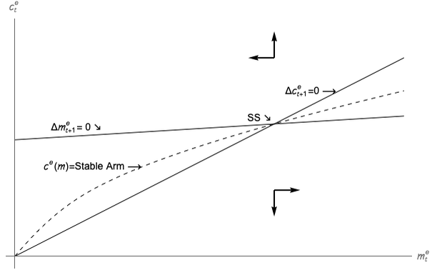
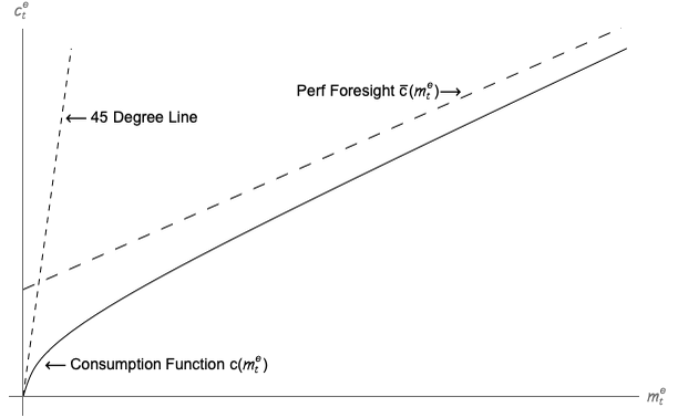
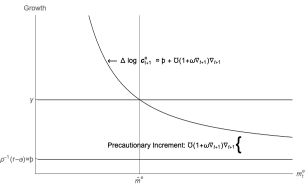

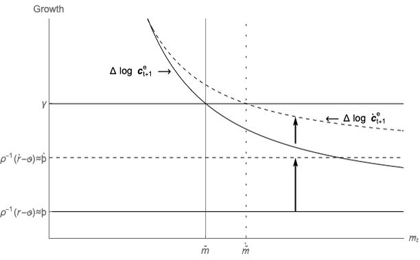

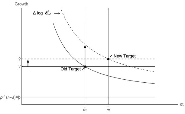
 On Consumption Function
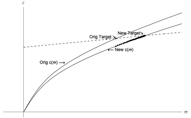
 Before and After
  Decline
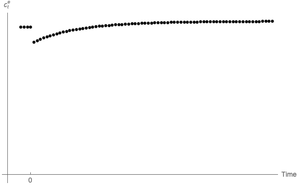
 Before and After
  Decline
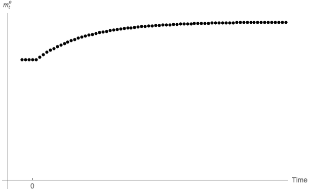
 Before and After
  Decline
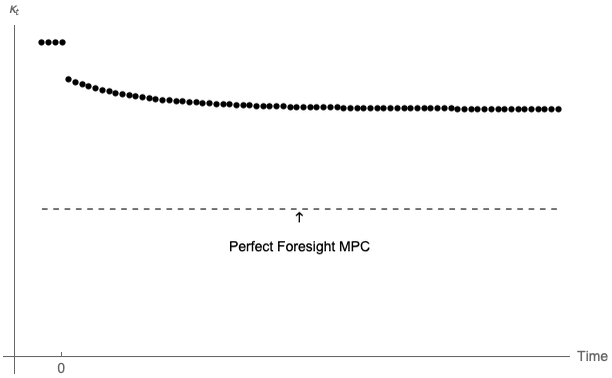
 in PE/SOE Economy Before and After
  Decline
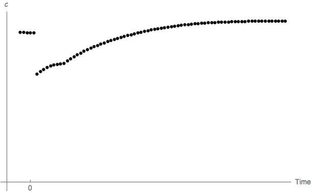
 in Stakeless PE/SOE Economy From Date 0