Dynamics of Wealth and Consumption:
New and Improved Measures for U.S. States
March 3, 2012
_____________________________________________________________________________________
Abstract
Case, Quigley, and Shiller (2005) persuasively argue that the well-known
conceptual difficulties in measuring aggregate “wealth effects” might be lessened
by the use of state-level data. Unfortunately, the data required for a convincing
implementation of their idea have been either virtually nonexistent (for financial
wealth) or of questionable quality (for consumption). Our main contributions
are to provide the first directly observed panel data on financial wealth
at the state level, and to construct improved measures of state-level
spending growth. Using these data, we estimate rudimentary “wealth effects”
regressions that find a strong relationship between twice-lagged housing
wealth growth and current spending growth, but we find no relationship
between lagged financial wealth growth and current spending growth.
1Zhou: xia_zhou@fanniemae.com, Federal National Mortgage Association, 3900 Wisconsin Ave, Washington,
DC 20016 2Carroll: ccarroll@jhu.edu, Department of Economics, 440 Mergenthaler Hall, Johns Hopkins
University, Baltimore, MD 21218, http://www.econ2.jhu.edu/people/ccarroll, and National Bureau of
Economic Research.
-
Keywords
-
housing wealth effect, financial wealth effect
-
JEL codes
-
E2, G1
1 Introduction
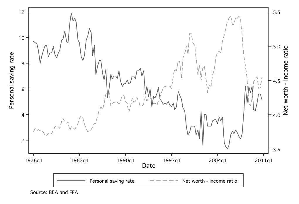
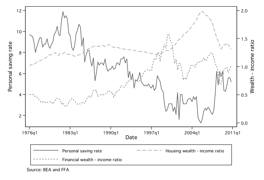
Macroeconomic forecasting models often incorporate a “wealth effect” which
asserts that movements in household net worth cause corresponding
movements in aggregate consumption. U.S. data showing a striking
negative relationship between the wealth-to-income ratio and the
personal saving rate (see Figure 1) are often presented in support of this
proposition, and statistical analysis finds a robust relationship between
aggregate wealth movements and subsequent household spending
growth.
But a skeptic could find plenty of reasons to doubt that this correlation reflects
causation from wealth movements to consumption or saving outcomes. First, the
association could reflect simultaneity. For instance, any shock to consumers’
optimism or pessimism could have an impact on housing prices, stock prices, and
consumption growth in the same direction. Second, endogeneity could also reflect
reverse causality of consumption on wealth (for example, a consumption boom
might bid up stock prices as expected profits rise). Finally, simple kinds of
measurement error could lead to the observed association. For example, suppose
that income  is measured with error. By construction, the personal saving
rate,
is measured with error. By construction, the personal saving
rate,  , will also be mismeasured in the same direction
as
, will also be mismeasured in the same direction
as  . At the same time, the measured wealth-income ratio
  will be biased in the opposite direction, generating a spurious negative
relationship.
will be biased in the opposite direction, generating a spurious negative
relationship.
In an effort to get around these problems, a substantial literature has turned to
micro data. But household-level data suffer from serious measurement
problems. There is a very limited choice of household-level data available
for carrying out such studies in the U.S. For instance, the Panel Study
on Income Dynamics (PSID) only measures food consumption, while
the Consumer Expenditure Survey (CEX) has detailed but noisy data
on household expenditures and poor financial information. The Survey
of Consumer Finances (SCF) provides no measure of consumption at
all.
An alternative approach, one that potentially avoids some of the problems
related to both aggregate and household-level data, is to use regional
data. First, if there is sufficient variation across regions, the endogeneity
problem might be mitigated. For instance, consider a region-specific shock
to consumers’ confidence, one that might also have a large impact on
the consumption behavior of households in the region. However, if a
well-integrated stock market exists, this region-specific shock might not have as
great an impact on stock prices of persons who live in the region as a
corresponding aggregate shock to confidence would have on aggregate stock
prices. Therefore, the endogeneity problem between local wealth and local
consumption is alleviated to some extent. Furthermore, it can be argued that
regional data provides more comprehensive and better measures of the
relevant variables than household-level data. Finally, regional data is
more likely to cover a longer time period and therefore allow for richer
dynamics.
Case, Quigley, and Shiller (2005) pioneered the estimation of wealth effects
using regional data. We improve on their efforts in several ways. Most notably,
after showing that CQS used a flawed method to construct state-level
financial wealth, we construct a new panel dataset of financial wealth
for U.S. states, using anonymous proprietary account-level records of
geographic wealth holdings. We will argue that our new financial wealth
dataset is much more accurate than existing alternative measures used
previously in the literature. Another contribution of this paper is to construct
a significantly improved state-level proxy for consumption data. Our
two new datasets are then combined to provide new estimates of how
household spending changes following movements in stock and housing
wealth.
The rest of the paper is organized as follows: Section 2 reviews the related
literature; Section 3 discusses the limitations of the currently available state-level
consumption and stock wealth datasets; Section 4 describes the newly
constructed data; and Section 5 presents the model specification and regression
results, then uses those results to calculate the estimated contribution of
disparate cross-state housing wealth movements to differences in the runup in
consumption spending (prior to 2008) and the subsequent decline (after 2008).
Some very rough calculations suggest that only a small portion of the
post-2008 decline in spending can be attributed to the effects of housing price
declines (though the estimated long lags in the housing wealth effect
suggest that spending weakness may continue for some time). Section 6
concludes.
2 Recent Evidence
The existing literature on whether the marginal propensity to consume
(MPC) differs out of different components of wealth is small. Davis and
Palumbo (2001b) compared the stock market wealth effect with the
non-stock-market wealth effect using U.S. aggregate data. The results, derived
from a cointegration analysis, are, however, sensitive to model specification. The
long-run effects of both types of wealth are estimated to be about the same (i.e.,
0.06 for stocks and 0.08 for non-stocks) when the level of variables is used. Using
logarithms, however, the results show an elasticity for non-stock wealth four
times greater than that for stock wealth; this implies that the MPC
out of non-stock wealth is at least twice as large as the MPC out of
stock wealth. Additionally, using aggregate data (though applying a
different method), Carroll, Otsuka, and Slacalek (2011) reported an
immediate MPC out of housing wealth of about 1.5 cents and an immediate
stock wealth MPC of 0.75 cents. This difference, however, is statistically
insignificant.
Levin (1998) appears to be the first study in the U.S. to use household-level
data to estimate the differential effect of housing and stock wealth. Using the
Retirement History Survey, Levin found that housing wealth has essentially no
effect on consumption. Out of eight spending categories, only three reported a
statistically significant difference between the respective coefficients for
liquid and housing wealth. This finding contradicts the studies using
aggregate data summarized above. A possible reason could be the fact
that every interviewee in the survey is at least 65 years old. If elderly
people tend to view housing wealth more as consumption than as an
investment item, their housing wealth effect will be lower than would
otherwise be the case. Using the CEX and SCF, Bostic, Gabriel, and
Painter (2009) find that, while incorporating all households in their sample,
there is no evidence for an important housing wealth effect. Among home
owners, however, the housing wealth elasticity is found to be consistently
significant and larger than the stock wealth elasticity. Their paper also
suggests different consumption behaviors for credit-constrained versus non
credit-constrained samples. Using household-level data in the U.K., Campbell
and Cocco (2007) found the response of household consumption to housing
prices is rather large and significant. They also provide evidence for the
heterogeneity of this response. More specifically, the estimated housing
price elasticity is as large as  for old home-owners but near zero
for young renters. Attanasio, Blow, Hamilton, and Leicester (2009),
however, found a larger relationship between consumption and house
prices for younger households. The authors then suggested that both
consumption and house prices are responding to some common factors.
Using a different British household-level dataset, Disney, Gathergood,
and Henley (2010) found a small housing wealth effect of
for old home-owners but near zero
for young renters. Attanasio, Blow, Hamilton, and Leicester (2009),
however, found a larger relationship between consumption and house
prices for younger households. The authors then suggested that both
consumption and house prices are responding to some common factors.
Using a different British household-level dataset, Disney, Gathergood,
and Henley (2010) found a small housing wealth effect of  after
controlling for financial expectations, without which the estimated housing
wealth effect would be significantly biased up. If simultaneity of this kind
can be found even in micro data, where it should be harder to find, it
appears to justify the concern with simultaneity problems using aggregate
data.
after
controlling for financial expectations, without which the estimated housing
wealth effect would be significantly biased up. If simultaneity of this kind
can be found even in micro data, where it should be harder to find, it
appears to justify the concern with simultaneity problems using aggregate
data.
The best known paper using geographical data is Case, Quigley, and
Shiller (2005). Using quarterly U.S. state-level data for 1982 through 1999,
the authors found a significant housing wealth elasticity of about  percent, but an economically negligible stock wealth elasticity under most
model specifications. When using a panel of annual data for 14 developed
countries, they found an even larger housing wealth elasticity, in the range of
percent, but an economically negligible stock wealth elasticity under most
model specifications. When using a panel of annual data for 14 developed
countries, they found an even larger housing wealth elasticity, in the range of
 percent. Nonetheless, under all cases, they found no evidence
for an important stock wealth effect. Case, Quigley, and Shiller (2011)
extended their state-level data up to 2009 and applied the same technique
to address the wealth effect question. Similar to their previous study,
the authors found significant and rather large housing wealth effect on
consumption and consistently found larger housing wealth effect than
stock wealth effect. However, after including data during
percent. Nonetheless, under all cases, they found no evidence
for an important stock wealth effect. Case, Quigley, and Shiller (2011)
extended their state-level data up to 2009 and applied the same technique
to address the wealth effect question. Similar to their previous study,
the authors found significant and rather large housing wealth effect on
consumption and consistently found larger housing wealth effect than
stock wealth effect. However, after including data during  ,
the recent housing market meltdown, the authors found that increases
and declines in the housing market have equally important effects on
consumer spending, which contradicts their previous findings. Bayoumi and
Edison (2003) used data for 16 industrial countries and found significant
wealth effects for most samples and periods. Their estimated housing
wealth effect was consistently larger than their estimated equity wealth
effect. Ludwig and Sløk (2002) found evidence contrary to the studies
cited above. Using annual data from 16 OECD countries, and taking
housing prices and stock market prices as proxies for their respective
wealth components, the authors reported an estimated stock wealth
elasticity twice the estimated housing wealth elasticity. Additionally, both
estimates were found to be positive and statistically significant. On the other
hand, Girouard and Blöndal (2001) also used OECD data, but were
unable to arrive at consistent results when comparing housing wealth
with financial wealth. Dvornak and Kohler (2003), using Australian
state-level data, found a larger stock wealth effect than housing wealth
effect.
,
the recent housing market meltdown, the authors found that increases
and declines in the housing market have equally important effects on
consumer spending, which contradicts their previous findings. Bayoumi and
Edison (2003) used data for 16 industrial countries and found significant
wealth effects for most samples and periods. Their estimated housing
wealth effect was consistently larger than their estimated equity wealth
effect. Ludwig and Sløk (2002) found evidence contrary to the studies
cited above. Using annual data from 16 OECD countries, and taking
housing prices and stock market prices as proxies for their respective
wealth components, the authors reported an estimated stock wealth
elasticity twice the estimated housing wealth elasticity. Additionally, both
estimates were found to be positive and statistically significant. On the other
hand, Girouard and Blöndal (2001) also used OECD data, but were
unable to arrive at consistent results when comparing housing wealth
with financial wealth. Dvornak and Kohler (2003), using Australian
state-level data, found a larger stock wealth effect than housing wealth
effect.
3 Limitations of existing state-level consumption and stock wealth
data
Case, Quigley, and Shiller (2005) relate state-level quarterly spending growth to
measures of quarterly state-level stock wealth and housing wealth for the
U.S. for the period 1982 through 1999, and Case, Quigley, and Shiller (2011)
extend that estimation to 2009. But serious problems afflict their measures of
both financial wealth and consumption.
3.1 Financial Wealth
No direct measures of state-level financial wealth data exist, so CQS had to
construct their own estimates. The best data they were able to find was
occasional information about state-level holdings of mutual funds. In order to
produce a measure of state-level stock wealth, CQS assumed that the ratio of
mutual funds holdings to holdings of other financial assets was identical across
states (and equal to the aggregate value of that ratio), which implies that the
distribution of financial wealth across states can be constructed using
the pattern of mutual fund holdings (for years in which mutual fund
holdings are available). CQS obtained the mutual fund data for the years
1986, 1987, 1989, 1991, 1993, 2008, and 2009. In the absence of data
for other years, they assumed a constant distribution of mutual fund
holdings across states for the period  and
and  .
During those years, then, movements in the stock wealth of each state
is assumed to mimic the movement of aggregate stock wealth. From
1999 to 2008, they assume that the ratio of mutual fund assets to total
assets increases linearly so that it matches the aggregate figure in 1999
and 2008. (2008-2009 is the only pair of adjacent years in which the
relevant data are available in both years to construct their measure without
interpolation).
.
During those years, then, movements in the stock wealth of each state
is assumed to mimic the movement of aggregate stock wealth. From
1999 to 2008, they assume that the ratio of mutual fund assets to total
assets increases linearly so that it matches the aggregate figure in 1999
and 2008. (2008-2009 is the only pair of adjacent years in which the
relevant data are available in both years to construct their measure without
interpolation).
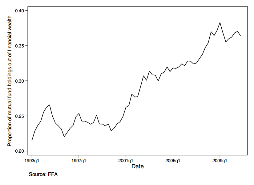
One aspect of their methodology, at least, is subject to test: Their assumptions
about the movements in the ratio of mutual fund holdings to total financial
wealth. Figure 2 plots mutual fund holdings from FFA over the same
period, and shows strong deviations from a linear increase in the ratio of
mutual fund holdings to total financial assets at the aggregate level.
Since aggregate data is the sum of state data, the CQS method must
be producing mismeasurements of the state-level financial wealth data
even if their assumption is correct that the ratio of mutual fund to total
financial assets is identical across states. In principle, mismeasurement of
a regressor tends to bias its coefficient toward zero; so an unfriendly
interpretation of the CQS finding that the ‘financial wealth effect’ is small
might be that this is because their measure of financial wealth changes is
noisy.
3.2 Consumption
To the best of our knowledge, there exist three distinct state-level sources of
consumption data – those used by Asdrubali, Sorensen, and Yosha (1996); Case,
Quigley, and Shiller (2005) and Case, Quigley, and Shiller (2011); and Garrett,
Hernàndez-Murillo, and Owyang (2004). Of these, only CQS utilized the data
to examine wealth effects. The consumption data used by Asdrubali,
Sorensen, and Yosha (1996), and CQS used estimates of retail sales
obtained from private sector sources. However, in both cases, the quality of
these data derived from the private sources is questionable. First, the
methodology used in the data construction is never explicitly revealed by
either private source. Second, retail sales are presented for states that
do not implement sales tax, which constitutes perhaps the single most
important source for calculating state retail sales after the Census Bureau
ceased reporting monthly retail sales by state, in 1997. Last but not
least, both sources vaguely note that important state-level variables
like wage and employment data are incorporated into the estimation of
retail sales. As a result, use of these data is likely to generate unreliable
estimations of the relationship between consumption and any variable
that is correlated with wages or employment. (For example, a finding
that ‘consumption growth is related to the predictable component of
wage growth,’ a classic test of the permanent income hypothesis, would
obviously be spurious if the measure of consumption was generated by
imputation from wage growth data; the vague descriptions of the private firms’
data construction methods suggest that this is more than a hypothetical
problem.)
Given these problems, we are skeptical of the empirical results of any study
that uses data from these private sources. (For considerably more discussion of
these sources and their doubtful properties, see Zhou (2010)).
More promising is the method of Garrett, Hernàndez-Murillo, and
Owyang (2004), who computed quarterly retail sales by dividing sales tax
revenue by the sales tax rate. In principle this could potentially yield a good
measure of state retail sales, and this method therefore provides the basis of the
measure of spending growth measure we use in this paper. One problem,
however, is that the sales tax revenues are occasionally measured with serious
errors; this results in observations with unreasonably large consumption
variations and apparent outliers. We carefully examined these events and found
that many of them could be explained, and many of those that could not be
explained were nevertheless obviously errors. Thus, our dataset “cleans up”
these outliers and thereby improves upon the data used in Garrett et. al.
(2004).
4 Data Description
This paper uses a panel dataset for  U.S. states as well as Washington,
D.C., at a semiannual frequency for the period 2001 through 2005. The
newly constructed datasets are for stock wealth and consumption at the
state level. Other important variables include after-tax labor income
and housing wealth. All are expressed in real per capita terms. There is
evidence that the new data are more comprehensive and accurate than
other existing alternatives. Some important findings will be discussed
in the rest of this section. More detailed discussions can be found in
Zhou (2010).
U.S. states as well as Washington,
D.C., at a semiannual frequency for the period 2001 through 2005. The
newly constructed datasets are for stock wealth and consumption at the
state level. Other important variables include after-tax labor income
and housing wealth. All are expressed in real per capita terms. There is
evidence that the new data are more comprehensive and accurate than
other existing alternatives. Some important findings will be discussed
in the rest of this section. More detailed discussions can be found in
Zhou (2010).
4.1 Stock wealth data
We obtained anonymous account-level records on financial wealth holdings at the
ZIP+4 Code level from a private company. At the end of each semiannual cycle,
that company collects data from more than  leading financial institutions in
its network. Reporting institutions include major banks, brokerage firms,
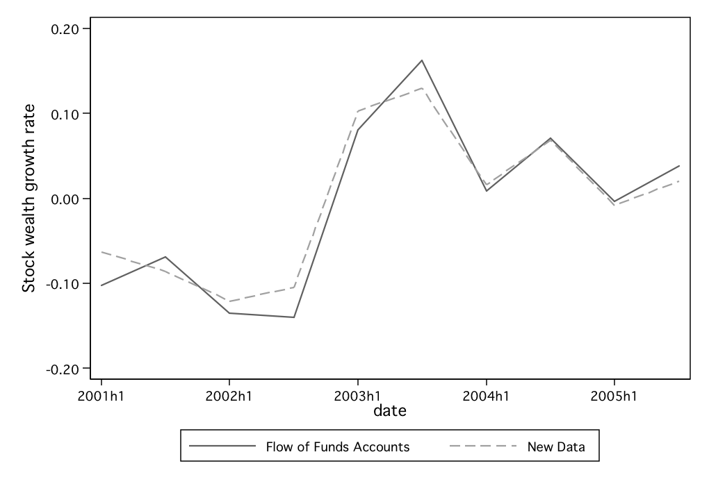
insurance companies and mutual fund dealers. Aggregate stock wealth growth
rates, as measured by both the Flow of Funds Accounts (FFA) and the new
dataset between 2000h1 and 2005h2, are presented in Figure 3. Despite using
completely different data sources, Figure 3 shows that the two series move
similarly to one another, suggesting that the new data is representative of the
nation as a whole.
leading financial institutions in
its network. Reporting institutions include major banks, brokerage firms,
insurance companies and mutual fund dealers. Aggregate stock wealth growth
rates, as measured by both the Flow of Funds Accounts (FFA) and the new
dataset between 2000h1 and 2005h2, are presented in Figure 3. Despite using
completely different data sources, Figure 3 shows that the two series move
similarly to one another, suggesting that the new data is representative of the
nation as a whole.
Stock market wealth is defined as the sum of directly and indirectly
held stocks and equity mutual funds (‘indirectly’ held assets are,
e.g., IRA and Keogh accounts). Stock wealth growth is constructed
using a consistent method for all 50 states plus the District of
Columbia.
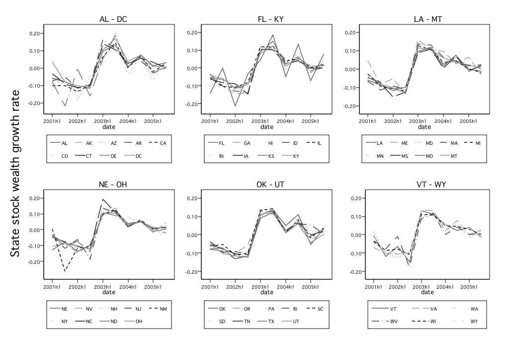
The geographic distribution of stock wealth growth is plotted in Figure 4. We
find similar patterns across states, something to be expected given the fact that
the U.S. stock market is so well integrated. Since there exists no alternative
state-level wealth data for comparisons, we use stylized facts about the U.S. to
understand if the state heterogeneity manifested in the figure reflects
reality.
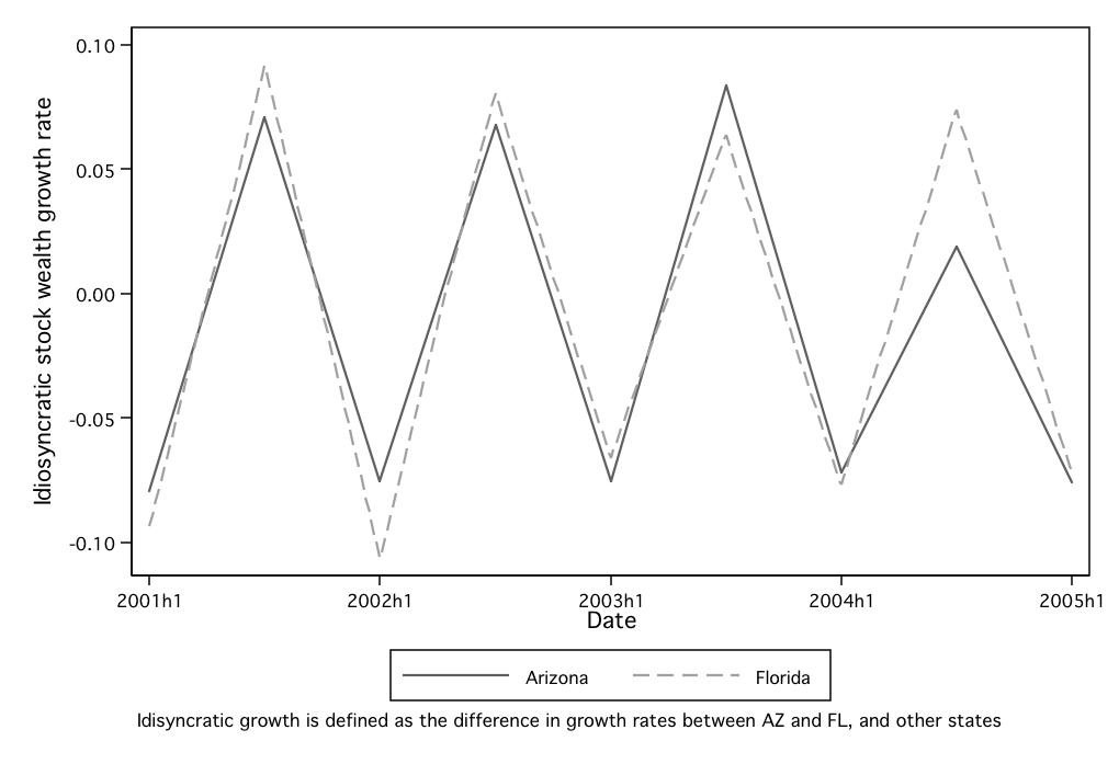
Florida and Arizona are the two states that have the highest percentage of
retired people. As reflected in Figure 4, their seasonal patterns also distinguish
them from other states. In order to better illustrate the differences, Figure 5
compares the stock wealth growth of Florida and Arizona with the average stock
wealth growth of the other states. It indicates that Florida and Arizona have a
much higher stock wealth growth rate than the other states during the second
half of each year, and a much lower stock wealth growth rate during the first half
of each year. This phenomenon might seem strange at first glance, but is actually
an outcome of the “snow-bird effect.” In the U.S., many retired people
tend to move to Florida and Arizona during the winter and then move
back to their permanent residences once the winter is over. If some such
individuals update their physical mailing addresses with their financial
institutions when they relocate, they effectively bring their assets along with
them.
Figures 5 therefore provide evidence that the data are indeed capable of
capturing state-level variations that are both meaningful and independent of
aggregate movements. (The patterns here also motivate our use of year-over-year
growth averages in our empirical work, to avoid seasonal patterns of the kind
identified here).
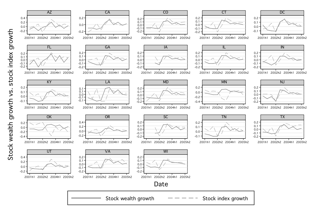
We exerted substantial effort to find any other measure of state-level financial
resources with which the new data could be compared, without great success.
The most plausible indicator is from Bloomberg, which reports local stock
indices for 23 states; the literature on the “home bias” of investments would lead
us to expect that the growth of this variable to be positively but not
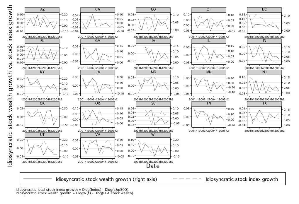
perfectly correlated with local stock wealth growth. Figure 6 presents the
correlation between the local stock index and local stock wealth, broken
down graphically. Out of the 23 calculated correlations, we find only 2
negative numbers. At the state-specific growth level, defined as state
growth minus the U.S. national component, there are still 15 positive
correlations. These facts further provide supporting evidence that the data
is correlated with the true distribution of stock market wealth across
states.
4.2 Consumption data
Since measures of personal consumption expenditure (PCE) at the state level are
not available in the U.S., retail sales are used as a proxy for consumption. In the
U.S., national retail sales account for roughly half of PCE, and The Retail Trade
Survey is probably the single most important source for the national
PCE estimation carried out by the Bureau of Economic Analysis (BEA).
Actually, for nonbenchmark-year estimates for most categories of PCE,
the retail sales series are used in the interpolation and extrapolation
process, as well as the “control total” calculation for each retail control
group.
These considerations provide us with a rationale for using retail sales in place of
consumption.
However, retail sales data are not directly available in the U.S. at the state
level. Following Garrett, Hernàndez-Murillo, and Owyang (2004), quarterly
state-level general sales tax revenues can be obtained from the Quarterly
Summary of State and Local Government Tax Revenue, published by the U.S.
Census Bureau. Together with general sales tax rates collected from various
sources,
state-level retail sales are computed by dividing the state general sales tax
revenue by the general sales tax rate. One limitation of this method is that
since 5 states do not have retail sales taxes, it can be applied only to 45
states and the District of Columbia. Nevada, however, is dropped in this
study because of its discontinued data report and obvious poor data
quality.
Strictly speaking, the computed retail sales are only one component of true
retail sales, as they exclude items that are either not subject to sales tax or are
part of special tax programs, i.e., liquor and cigarettes. Furthermore, there is
unquestionably serious measurement error in the computed retail sales from a
host of sources (including, for example, imperfect measurement of changes in
retail sales tax rates and the distribution of tax rates across categories of goods).
However, we discovered that 12 states actually directly report (taxable) retail
sales for the same period during which state-level stock wealth data is
available.
These measures are more comprehensive than our computed measure of retail sales,
as they either include all consumption items (such as when government-reported
gross retail sales are used) or at least include those items that are part of special tax
programs.
Furthermore, these government-reported measures should be
more accurate and reliable than the computed ones, since local
governments have access to more information regarding their own
sales tax system and tax collection practices than other people
do. 
Ideally, government-reported (taxable) retail sales should be used as a measure
of consumption. However, since they are only available for a limited
number of states, this paper compiles three sets of consumption data
according to the quality of the retail sales data. The first one includes those
12 states that have government-reported retail sales or taxable retail
sales; it is categorized as “Best Data.” The second set is called “Good
Data,” which is the computed retail sales with outliers taken care of. The
third set is called “Combined Data,” and is “Best Data” combined with
“Good Data” whenever the former is not available. Table 1 presents the
summary statistics of each set of consumption data. Please refer to the third
chapter of Zhou (2010) for a more detailed discussion of the consumption
data.
4.3 Data from other sources
Other important variables used in this paper include quarterly after-tax labor
income and housing wealth. After-tax labor income is calculated following
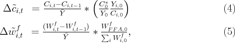
Lettau and Ludvigson (2001). The formula used to construct state-level
housing wealth is similar to the one adopted by CQS, and is given as
follows:
 where
where  is the value of the owner occupied housing wealth for state
  ;
;  is the home ownership rate, taken from the Census Bureau;
  is the
weighted repeat sales housing price index, taken from the Federal Housing
Finance Agency (FHFA); and
is the
weighted repeat sales housing price index, taken from the Federal Housing
Finance Agency (FHFA); and  is the average home price for 1999, taken
from the 2000 Census. Summary statistics of all newly constructed data series
are presented in Table 1.
is the average home price for 1999, taken
from the 2000 Census. Summary statistics of all newly constructed data series
are presented in Table 1.
4.4 Data issues
One important data issue arises here. As mentioned above, all variables except
the stock market wealth are available at quarterly frequencies. To make them
analogous to the stock market wealth, this paper takes their means over
the quarters for each half-year, thus converting them into semiannual
frequencies.
The dataset, however, features evident and sizable seasonal patterns at the
semiannual frequency, especially for the constructed consumption data. We made
a considerable effort at removing these seasonal patterns in a consistent fashion,
but were unable to do so at the semiannual frequency. This is largely because of
the heterogeneity of seasonal patterns across states and the relatively short time
horizon. (Many state governments recommend using longer time spans for more
reliable trends.) It should be recognized that measures of taxable sales (or
revenue) at higher frequencies could be unrepresentative for the purpose of
comparison. This is because of timing errors over the year-long period. The
above consideration persuaded us to use annual growth rates so as to eliminate
seasonal effects, at the cost of fewer observations and thus a reduced regression
power.
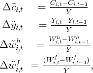
Additionally, to avoid a time aggregation problem, annual averages are not
used to calculate growth rates. Instead,  is computed as the log difference
between consumption for the first half of year
is computed as the log difference
between consumption for the first half of year  and for year
  . The first
half was chosen in consideration of the fact that the state fiscal year ends
on June 30th. It is arguable that data collected towards the end of a
fiscal year is more accurate than data collected at any other time of
year.
. The first
half was chosen in consideration of the fact that the state fiscal year ends
on June 30th. It is arguable that data collected towards the end of a
fiscal year is more accurate than data collected at any other time of
year.
4.5 Another look at the new data
Since this paper relies heavily on the two newly constructed datasets, before
examining wealth effects, we report a simple regression of the form
where  denotes the growth rate of a variable, i.e., the log difference of the
variable in real per capita terms. Equation 1 is a simple description of the data
without taking into consideration simultaneity and aggregation problems. Table
3 reports the results for all three datasets. It shows that income growth is
the one variable that consistently has the largest and most significant
coefficient. Perhaps the most interesting finding is that there is evidence
that consumption positively correlates with the growth rates of both
housing wealth and stock wealth when they are regressed separately.
Conversely, whenever income growth is included, their respective coefficients
become much less significant, in connection with the reduced sizes. The
data archive that can produce all results in this study is available from
http://www.econ2.jhu.edu/people/ccarroll/papers/zcWandCdynByState.zip.
denotes the growth rate of a variable, i.e., the log difference of the
variable in real per capita terms. Equation 1 is a simple description of the data
without taking into consideration simultaneity and aggregation problems. Table
3 reports the results for all three datasets. It shows that income growth is
the one variable that consistently has the largest and most significant
coefficient. Perhaps the most interesting finding is that there is evidence
that consumption positively correlates with the growth rates of both
housing wealth and stock wealth when they are regressed separately.
Conversely, whenever income growth is included, their respective coefficients
become much less significant, in connection with the reduced sizes. The
data archive that can produce all results in this study is available from
http://www.econ2.jhu.edu/people/ccarroll/papers/zcWandCdynByState.zip.
5 Regressions
5.1 Wealth effect estimation
Many studies in the current literature, particularly those that focus on the immediate
response of consumption to wealth, adopt regressions similar to those used in
Equation 1.
However, even if simultaneity problems did not exist, such regressions would not
yield straightforward measures of wealth effects, since they only report the
contemporaneous growth correlation between consumption and wealth.
Worse, in this specification it is not straightforward to test the interesting
hypothesis that stock and housing wealth effects are of equal size (which is
assumed whenever an overall “wealth effect” is estimated, but may not be
true).
In order to solve this problem, this paper adopts an approach similar to that
employed by Carroll, Otsuka, and Slacalek (2011); those authors use
the ratio of the change in each variable relative to an initial level of
consumption spending. Here, we use average aggregate labor income between
 and
and  as the denominator instead. Specifically, if we define
where  is the state after-tax labor income at 2000h1, then the following
regression would (in the absence of simultaneity problems) produce direct measures of the
MPC out of the changes in housing wealth and stock wealth.
is the state after-tax labor income at 2000h1, then the following
regression would (in the absence of simultaneity problems) produce direct measures of the
MPC out of the changes in housing wealth and stock wealth.
As with Equation 1, Equation 2 is subject to serious endogeneity problems,
and thus must be considered as simply another description of the data. Table 4
indicates that under this model specification, income change is still the most
correlated variable with respect to consumption.
In order to address the endogeneity and simultaneity problems that Equation 2
is subject to, we briefly revisit classic consumption theory. The relationship
between consumption and wealth and income can be described by the
Life-Cycle/Permanent Income Hypothesis. Specifically, a consumer wants to
subject to the budget constraint, where  is the time preference, and
  is
the utility function. If the utility function takes a quadratic form as assumed in
Hall (1978), it can be easily shown that, under certain conditions, consumption
will follow a random walk, i.e., Thus, the theory implies that consumption responds to unexpected shocks only.
In other words, information known to consumers at the time when consumption
choices are made cannot have any predictive power for consumption changes in
any future periods.
is
the utility function. If the utility function takes a quadratic form as assumed in
Hall (1978), it can be easily shown that, under certain conditions, consumption
will follow a random walk, i.e., Thus, the theory implies that consumption responds to unexpected shocks only.
In other words, information known to consumers at the time when consumption
choices are made cannot have any predictive power for consumption changes in
any future periods.
The random walk proposition, therefore, can help us address the endogeneity
and simultaneity problem, as it suggests that current consumption growth would
not be correlated with any lagged wealth growth. Nevertheless, time aggregation
and measurement error could cause current consumption changes to correlate
with once lagged income and wealth changes, even if the PIH holds true.
Aggregation also matters when the PIH holds in continuous time, and
the measures of consumption are based on time averages. Under this
situation, changes in time-averaged consumption will have nonzero first
order serial correlations; this will lead to nonzero correlations between
changes in consumption and once-lagged variables. It is also easy to
prove that measurement errors in the consumption level could cause
measured consumption changes that correlate with once-lagged explanatory
variables.
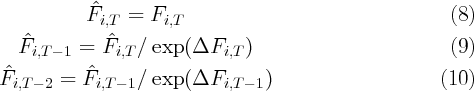
Given the above considerations, the following equation is
employed to see if we can detect delayed effects of wealth
changes:

Equation 3 employs twice-lagged independent variables, and thus gives a
rudimentary estimate of current MPCs out of changes in housing wealth and
stock wealth that occurred two periods prior, which would be zero in the random
walk model.
There are, however, two minor modifications that need to be made. First, what
 captures here is not the real personal consumption for state
  , but the
state’s taxable retail sales. Thus, using
, but the
state’s taxable retail sales. Thus, using  , the estimation of Equation 3
actually yields the effect of changes in wealth on taxable retail sales. To gauge
the approximate change in real consumption, it is assumed that initial
state consumption can be determined by
, the estimation of Equation 3
actually yields the effect of changes in wealth on taxable retail sales. To gauge
the approximate change in real consumption, it is assumed that initial
state consumption can be determined by  , where
  and
and  are aggregate personal consumption expenditure and after-tax
labor income, respectively. In addition, we assume that the ratio of retail
sales to real consumption holds constant over time, i.e.,
are aggregate personal consumption expenditure and after-tax
labor income, respectively. In addition, we assume that the ratio of retail
sales to real consumption holds constant over time, i.e.,  .
Therefore, changes in state consumption can be measured roughly by
.
Therefore, changes in state consumption can be measured roughly by
The
same problem arises when measuring stock wealth. Thus, it is assumed for all
states and time periods that 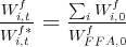 , where
  denotes the real state
stock wealth at time
denotes the real state
stock wealth at time  .
.
Therefore, if we redefine
the
regression of Equation 3 ends up reporting approximate estimates of the MPC
out of changes in housing wealth and stock wealth.
Table 5 summarizes the results of our estimations using Equation 3. It
indicates that all three datasets report similar results, with the exception that
none of the estimations from “Best Data” is statistically significant. Given the
small sample size of the “Best Data” sample, this is perhaps not too
surprising.
Table 5 shows that the coefficients of income changes are all positive and large.
It therefore implies that income changes have a fairly big impact on
consumption, despite the two-year lag. This, however, contradicts the random
walk theory as predicted by the Permanent Income Hypothesis.
The wealth effect from lagged changes in financial wealth, on the other hand, is
found to be both statistically insignificant and economically negligible. This
finding is consistent with Dynan and Maki (2001), who found that the impact of
stock wealth on consumption very quickly becomes apparent, and any lagged
change in stock wealth beyond 9 months does not have any significant effect on
consumption.
However, we observe highly significant and large coefficients for housing wealth
in two out of the three datasets. Additionally, all three datasets indicate an MPC
out of housing wealth changes that occurred two years prior around the
neighborhood of  cents.
There are several reasons why the response to housing wealth shocks may be
slower than the response to financial wealth shocks. Unlike stock prices
that can be easily tracked daily online or in newspapers, house prices
might be difficult to observe accurately or regularly. Homeowners might
be less aware of short-run changes in house prices and it might take
a homeowner a while to realize that his/her house price has changed.
Additionally, the cost of realizing capital gains on housing wealth is lumpy. As a
result, the response to housing wealth growth is not likely to be entirely
contemporaneous.
What is more interesting is that the difference between the housing wealth
effect and the stock wealth effect is found to be statistically significant
for “Good Data,” and on the verge of being significant for “Combined
Data.”
5.2 A habit formation test
A method for formalizing the sluggishness of the response of consumption to
changes in wealth was proposed by Carroll, Otsuka, and Slacalek (2011)
(henceforth ‘COS’), who show how to derive “eventual” wealth effects implied by
serial correlation in consumption growth. The basic idea is, if there is evidence of
habit formation, consumption growth will be serially correlated. Thus, any
impact that wealth changes have on consumption could be delivered
through the serial correlation of consumption growth. The eventual wealth
effect then can be derived by dividing the short run wealth effect by one
minus the habit formation coefficient. We attempt to test this method
of describing the consumption process using the equation derived by
COS:
 | (6) |
where the coefficient  is expected to indicate the strength of habit
formation.
is expected to indicate the strength of habit
formation.
Table 6 reports the estimations using Equation 6. Using currently
available state-level instruments, the results provide no evidence of habit
formation.
This could be because of the short time horizon of the data, and the
corresponding weakness of IV techniques like the one employed for this
test.
5.3 Post 2005
The U.S. economy entered a serious downturn in 2007 and is currently going
through a weak recovery. Therefore, it would be illuminating if we can conduct a
wealth-effect analysis using state-level data post 2005. State-level financial
wealth data, however, is currently only available through 2005. As a result, our
analysis in this section is performed without financial wealth growth. This is
arguably valid since financial wealth growth was found insignificant in previous
sections.
Similar to Table 3 and 4, Table 7 and 8 describe the data between 2001 and
2009, and present the test of structural break after 2005. It shows that both
income and housing wealth growth are positively and significantly correlated
with concurrent consumption growth. The null hypothesis of equal correlation
between consumption and income and/or housing wealth before and after
2005, however, is rejected under most scenarios. More interestingly, new
data tends to present a higher correlation between consumption and
income/housing wealth after 2005. Liquidity constraints might be a possible
reason that income and wealth are more correlated with consumption during a
recession.
Employing Equation 3, Table 9 repeats the wealth effect analysis without
financial wealth growth. Neither income nor housing wealth effect is found to be
significant. Furthermore, all three datasets show a negative coefficient for
housing wealth growth, indicating that consumption will decline in reaction to
increases in housing wealth two years ago. An obvious explanation is that the
two-year lag is too long if there is a bubble that inflates and then bursts, and if
there are immediate and once-lagged effects of housing wealth changes on
consumption that are larger than the twice-lagged effects. Housing price bubbles
and thus rapid increases in housing wealth occurred before the housing market
breakdown is the exact reason why the economy took a sharp turn in
2007.
The rest of this section is inspired by the work of Mian and Sufi (2011), who
study the patterns of household debt at the county level from 2002 to 2007, and
investigate how they are correlated with the following economic recession and
recovery. They find that not only did high household debt counties experience
larger declines in prices during the recession, but they also recover more slowly
after the recession. Employing their methodology, we take the 6 states that had
the highest house price growth during 2001-2006, then show the subsequent
behavior of house prices and consumption for 2007-2009. We do the same
thing for the 6 states having the lowest housing wealth growth between
2001-2006.
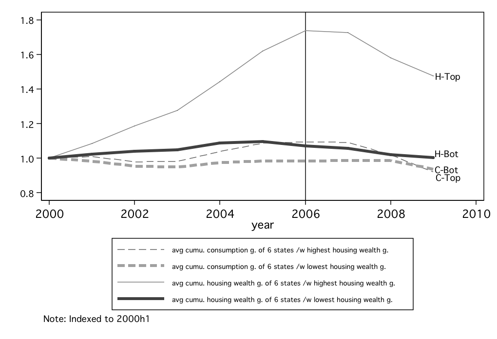
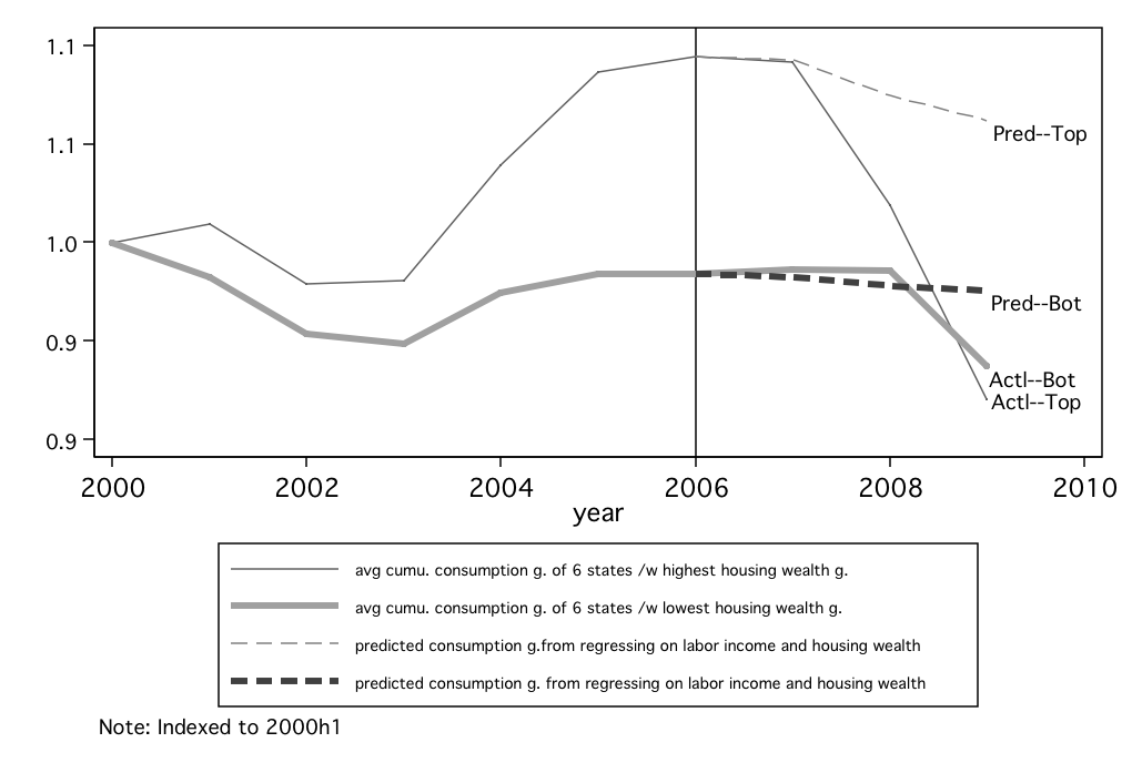
Figure 9 compares consumption and housing wealth, both indexed to 2000h1,
for the top and bottom 6 states during 2001-2006. The figure reflects the
well-known fact that housing wealth growth was highly heterogeneous across
states. The top 6 states experienced a sharp increase in housing wealth up to
2006 and experienced an equally sharp decline in housing wealth starting 2007.
On the other hand, the bottom 6 states show a much smoother housing wealth
growth path through the whole period. Figure 9 further shows that consumption
of both high and low housing wealth growth states contracted in 2001-2003,
likely due to the recession that started in 2001. Nevertheless, consumption of the
top 6 states with high housing wealth growth was rapidly increasing
as the real estate bubble was forming. In contrast, consumption of the
bottom 6 states only grew slightly as the housing market was booming
nationwide. By the time when national housing price peaked, consumption
of the top 6 states has been about  percent higher than its level
in 2000. But the bottom 6 states were still inching toward their 2000
level.
percent higher than its level
in 2000. But the bottom 6 states were still inching toward their 2000
level.
The observations above lead to an interesting question: Given what we knew
from the 2001-2006 estimates, how well would we have been able to predict
consumption declines after 2006 in the two groups of states had we known the
housing wealth and income changes they would experience over 2007-2009? In
other words, what fraction of the consumption declines after 2006 can be
associated with the concurrent housing wealth and income changes? (We freely
admit that this association cannot properly be interpreted as causal, for all the
reasons articulated in the introduction).
To address this question, we start by regressing consumption growth,  ,
on a time dummy, income growth, and housing wealth growth,
,
on a time dummy, income growth, and housing wealth growth,  , using
data between 2001-2006. We then predict consumption growth for 2007-2009 by
setting the intercept term to be zero. Figure 10 compares the actual and
predicted consumption growth for the top and bottom 6 states. It shows that the
top 6 states experienced an immediate drop in consumption as soon as the
housing market turned south in 2007, and continued with a sharp decline in
2008 as the subprime crisis intensified. Table 10 further shows, however,
that of the cumulative decline in consumption from 2006 to 2009, only
about
, using
data between 2001-2006. We then predict consumption growth for 2007-2009 by
setting the intercept term to be zero. Figure 10 compares the actual and
predicted consumption growth for the top and bottom 6 states. It shows that the
top 6 states experienced an immediate drop in consumption as soon as the
housing market turned south in 2007, and continued with a sharp decline in
2008 as the subprime crisis intensified. Table 10 further shows, however,
that of the cumulative decline in consumption from 2006 to 2009, only
about  percent can be ‘explained’ by the declines in income and
housing wealth. On the other hand, Figure 10 shows that states with the
bottom housing wealth growth hardly experienced any major consumption
contraction until 2009, when the subprime crisis had spread to non-subprime
areas and other industries. This nicely matches findings by Mian and
Sufi (2010) who find that spending on motor vehicles in non-housing-boom
states did not collapse until 2009, while motor vehicle purchases began
declining considerably earlier in the states that had a housing bubble then
bust. Together, these points suggest that, while problems in the housing
market may have been an important trigger for the 2008-2009 crisis, the
precipitous drop in consumption spending in that period went well beyond
what would have been expected just from the loss of housing wealth and
income.
percent can be ‘explained’ by the declines in income and
housing wealth. On the other hand, Figure 10 shows that states with the
bottom housing wealth growth hardly experienced any major consumption
contraction until 2009, when the subprime crisis had spread to non-subprime
areas and other industries. This nicely matches findings by Mian and
Sufi (2010) who find that spending on motor vehicles in non-housing-boom
states did not collapse until 2009, while motor vehicle purchases began
declining considerably earlier in the states that had a housing bubble then
bust. Together, these points suggest that, while problems in the housing
market may have been an important trigger for the 2008-2009 crisis, the
precipitous drop in consumption spending in that period went well beyond
what would have been expected just from the loss of housing wealth and
income.
6 Conclusion
This paper’s main contribution is to construct and describe two panel datasets:
One for financial wealth for U.S. states for 2000-2005, constructed from
anonymous proprietary account-level records of geographic wealth holdings, and
one for state-level consumption data, constructed using data on retail sales tax
revenues from the Census of State Governments (and, for some states, from
state-level estimates of retail sales); and to argue that these datasets are
substantially better than those that have been used by previous authors. We
then combine these datasets to provide new estimates of the relationship
between spending growth and current and lagged changes in stock wealth
and housing wealth. Consistent evidence is found for large but sluggish
housing wealth effects. Based on the results from our new approach,
two out of the three datasets indicate that the MPC out of a one dollar
change in two-year lagged housing wealth is about  cents. In addition,
the twice-lagged income change is also found to be strongly related to
the current consumption change. Both findings lead to the rejection of
the random walk model of consumption. Furthermore, a statistically
insignificant and economically small stock wealth effect is found for almost all
specifications, although large standard errors mean that the differences of
the financial wealth effect from housing wealth effects are statistically
insignificant.
cents. In addition,
the twice-lagged income change is also found to be strongly related to
the current consumption change. Both findings lead to the rejection of
the random walk model of consumption. Furthermore, a statistically
insignificant and economically small stock wealth effect is found for almost all
specifications, although large standard errors mean that the differences of
the financial wealth effect from housing wealth effects are statistically
insignificant.
In addition, the paper finds evidence for a strong association between
consumption and housing wealth declines in the period after the real estate
bubble burst; the states with the biggest housing wealth decline experienced
substantially larger declines in consumption spending. Our results also lend
tentative further support to the proposition asserted in CQS, in Carroll, Otsuka,
and Slacalek (2011), and elsewhere that movements in housing wealth and
financial wealth have different effects, with housing wealth changes apparently
exerting a large influence on household spending even two years after the
impulse. In addition to their salience for explaining recent events, these results
might also help explain the strength of consumption following the bursting of the
stock market bubble at the end of the  s: at the same time the
stock bubble was bursting, housing wealth had shown substantial gains,
and with a larger and more sluggish MPC might have been sufficient to
explain the strength of household spending in that era (in addition to its
weakness recently); see Figure 11 in the appendix for a breakdown of the
movements in wealth between financial and nonfinancial that supports this
story.
s: at the same time the
stock bubble was bursting, housing wealth had shown substantial gains,
and with a larger and more sluggish MPC might have been sufficient to
explain the strength of household spending in that era (in addition to its
weakness recently); see Figure 11 in the appendix for a breakdown of the
movements in wealth between financial and nonfinancial that supports this
story.
Figure 1: The saving rate versus the net worth - income ratio
Figure 2: Mutual fund holdings at the aggregate level
Figure 3: New data versus the Flow of Funds Accounts
Figure 4: Stock wealth growth rates across states: 
Figure 5: Snow bird effect
Note: The sharp seasonal fluctuations in wealth in Florida and Arizona likely reflect a “snow bird” effect, as wealthy
retirees move in and out of these states on a seasonal basis.
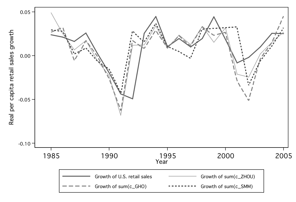
Figure 7: The sum of state retail sales measures versus U.S. aggregate retail sales
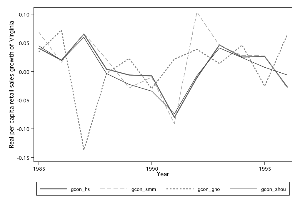
Figure 8: Virginia:  versus
  ,
,  , and
, and 
Figure 9: Housing wealth growth vs. consumption growth: 6 states with the
highest/lowest housing wealth growth during 2001-2006
Figure 10: Actual vs. predicted consumption growth: 6 states with the highest/lowest
housing wealth growth
Table 3: Data description: 
| Good Data
|
|
|
|
|
|
|
|
|
|
|
|
|
|
|
|
|
| | (1) | (2) | (3) | (4) | (5) | (6) | (7)
|
 | 1.009 | | | 0.989 | 0.971 | | 0.956 |
| | (0.246) | | | (0.251) | (0.254) | | (0.258) |
 | | 0.112 | | 0.059 | | 0.095 | 0.053 |
| | | (0.086) | | (0.085) | | (0.086) | (0.085) |
 | | | 0.093 | | 0.039 | 0.086 | 0.036 |
| | | | (0.055) | | (0.053) | (0.055) | (0.054) |
| Obs. | 180 | 180 | 180 | 180 | 180 | 180 | 180 |
 | 0.261 | 0.188 | 0.194 | 0.258 | 0.259 | 0.194 | 0.256 |
Partial  | 0.091 | 0.002 | 0.009 | 0.088 | 0.088 | 0.009 | 0.085 |
|
|
|
|
|
|
|
|
|
|
|
|
|
|
|
|
| |
| Combined Data
|
|
|
|
|
|
|
|
|
|
|
|
|
|
|
|
|
| | (1) | (2) | (3) | (4) | (5) | (6) | (7)
|
 | 1.054 | | | 1.028 | 0.983 | | 0.964 |
| | (0.21) | | | (0.21) | (0.216) | | (0.217) |
 | | 0.131 | | 0.076 | | 0.107 | 0.065 |
| | | (0.083) | | (0.078) | | (0.082) | (0.078) |
 | | | 0.128 | | 0.074 | 0.121 | 0.07 |
| | | | (0.05) | | (0.049) | (0.05) | (0.049) |
| Obs. | 180 | 180 | 180 | 180 | 180 | 180 | 180 |
 | 0.368 | 0.287 | 0.301 | 0.368 | 0.372 | 0.303 | 0.371 |
Partial  | 0.12 | 0.007 | 0.027 | 0.12 | 0.126 | 0.03 | 0.124 |
|
|
|
|
|
|
|
|
|
|
|
|
|
|
|
|
| |
a. Partial  refers to the proportion of variance explained by all variables other than the year dummies.
b. Standard errors in parenthesis. {*, **, ***} = significant at the {10%, 5%, 1%} level.
Table 7: Data description using data up to 2009: 
a. Partial  refers to the proportion of variance explained by all variables other than the year dummies.
b. Standard errors in parenthesis. {*, **, ***} = significant at the {10%, 5%, 1%} level.
c. F-Test and P-val is for the test of equal income and house wealth effect for the periods before and after 2005.
Table 10: Actual  vs. predicted
  for top and bottom states
A Stock Wealth Data
The data used in this paper were constructed during the author’s part-time
employment at a private company over two years. All financial data feeds are
provided as anonymous, ZIP Code data by product type. Absolutely no
non-public, personally identifiable information on U.S. households have been
used in this study.
Code data by product type. Absolutely no
non-public, personally identifiable information on U.S. households have been
used in this study.
Once the ZIP+4 Code level data is received by the private company, for ZIP+4
codes with fewer than  households, the data are joined and averaged with
other ZIP+4 Codes to ensure a minimum household count of
households, the data are joined and averaged with
other ZIP+4 Codes to ensure a minimum household count of  per ZIP+4
code. The average value is then imputed identically back down to the
affected ZIP+4 Codes. The rules utilized to perform the joining and
averaging are complex and based on geographical proximity and other
factors.
per ZIP+4
code. The average value is then imputed identically back down to the
affected ZIP+4 Codes. The rules utilized to perform the joining and
averaging are complex and based on geographical proximity and other
factors.
The names of the financial institutions reporting to the private company are
suppressed and cannot be revealed. However, it should be noted that the number
of reporting institutions changes over time. Hence, the biggest concern with
constructing the stock wealth data is the possibility that the variations in wealth
are caused by reasons other than the wealth holding variations of the
state residents. To minimize this problem, we expended a great deal of
effort keeping track of all mergers and institutions’ membership in the
network.
The formation of a consistent source of financial data over time was
performed at the state level. Thus, I could construct a common group of
reporting institutions for every TWO ADJACENT CYCLES. So the growth
rates could be calculated as the log difference of two adjacent values on
a rolling basis. Specifically speaking, for growth rate of stock wealth
for state  at time
  , we summed up the assets by those institutions
reporting at both
, we summed up the assets by those institutions
reporting at both  and
and  for state
  , and then I took the log
difference.
, and then I took the log
difference.
Specifically, suppose  is the total amount of stock wealth reported at time
 for state
  by institution
  .
.  is the set of all institutions reporting at
time
is the set of all institutions reporting at
time  for state
  . So
. So  is the set of all the institutions
reporting for state
is the set of all the institutions
reporting for state  at both time
  and
and  . Therefore,
  ,
the growth rate of stock wealth of state
,
the growth rate of stock wealth of state  at time
  is defined as:
where  .
.
After obtaining the correct growth rates, total stock market wealth for each
state were imputed backward as
where  and
and  .
.
Real stock wealth per capita is defined as
where  is the consumer price index at time
  and
and  is the
population of state
is the
population of state  at time
  . Therefore, growth rate of real stock wealth per
capita is calculated as:
. Therefore, growth rate of real stock wealth per
capita is calculated as:
B Results using the elasticity method
Many papers in the literature have estimated wealth effects by adopting the
elasticity method. Consequently, we then investigate the respective housing
wealth and stock wealth effects by estimating the following equation, as with
most related studies:
Table 11 reports the regression results from Equation 13 for all three sets of
consumption data. The findings are roughly consistent across the three
datasets.
The most outstanding and robust finding is the large coefficient for lagged
housing wealth. The stock wealth effects reported in Table 11 are all statistically
insignificant. Furthermore, in 2 of the 3 estimations, the size of the stock
wealth effect is economically small. The hypotheses of equal housing
wealth and stock wealth coefficients are, however, accepted in 2 out of 3
estimations.
Table 11: Results for the elasticity method
Figure 11: The saving rate versus the wealth - income ratio
References
ANTONIEWICZ, ROCHELLE L. (2000): “A Comparison of the
Household Sector from the Flow of Funds Accounts and the Survey of,”
Discussion paper, Federal Reserve Board.
ARON, JANIE, JOHN V. DUCA, JOHN MUELLBAUER, KEIKO
MURATA, AND ANTHONY MURPHY (2010): “Credit, Housing Collateral
and Consumption: Evidence from the UK, Japan and the US,” Working
Paper 1002, Federal Reserve Bank of Dallas.
ARON, JANINE, AND JOHN MUELLBAUER (2006): “Housing Wealth,
Credit Conditions and Consumption,” Centre for the Study of African
Economies Series WPS 2006-08, University of Oxford.
ASDRUBALI, PIERFEDERICO, BENT SORENSEN, AND OVED YOSHA
(1996): “Channels of interstate risksharing: United States 1963-1990,”
Quarterly Journal of Economics, 111, 1081–1110.
ATTANASIO, ORAZIO P., LAURA BLOW, ROBERT HAMILTON, AND
ANDREW LEICESTER (2009): “Booms and Busts: Consumption, House
Prices and Expectations,” Economica, 76(301), 20–50.
BAYOUMI, TAMIM, AND HALI EDISON (2003): “Is Wealth Increasingly
Driving Consumption,” DNB Staff Reports (discontinued) 101,
Netherlands Central Bank.
BERTAUT, CAROL (2002): “Equity Prices, Household Wealth, and
Consumption Growth in Foreign Industrial Countries: Wealth Effects
in the 1990s,” International Finance Discussion Papers 724, Board of
Governors of the Federal Reserve System.
BOSTIC, RAPHAEL, STUART GABRIEL, AND GARY PAINTER (2009):
“Housing Wealth, Financial Wealth, and Consumption: New Evidence
from Micro Data,” Regional Science and Urban Economics, 39, 79–89.
BYRNE, JOSEPH P., AND E. PHILIP DAVIS (2003): “Disaggregate
Wealth and Aggregate Consumption: an Investigation of Empirical
Relationships for the G7,” Oxford Bulletin of Economics and Statistics,
65(2), 197–220.
CAMPBELL, JOHN Y., AND JOAO F. COCCO (2007): “How Do House
Prices Affect Consumption? Evidence From Micro Data,” Journal of
Monetary Economics, 54(3), 591–621.
CAMPBELL, JOHN Y., AND N. GREGORY MANKIW (1989):
“Consumption, Income and Interest Rates: Reinterpreting the Time
Series Evidence,” in NBER Macroeconomics Annual, ed. by Olivier J.
Blanchard, and Stanley Fischer, Cambridge, MA. MIT Press.
CARDARELLI, ROBERTO, DENIZ IGAN, AND ALESSANDRO REBUCCI
(2008): “The Changing Housing Cycle and the Implications for Monetary
Policy,” in World Economic Outlook, chap. 3. Washington: International
Monetary Fund.
CARROLL, CHRISTOPHER D., MISUZU OTSUKA,
AND JIRI SLACALEK (2011): “How Large Are Housing
and Financial Wealth Effects? A New Approach,”
Journal of Money, Credit and Banking, 43(1), 55–79,
http://www.econ2.jhu.edu/people/ccarroll/papers/cosWealthEffects/.
CASE, KARL E., JOHN M. QUIGLEY, AND ROBERT J. SHILLER
(2005): “Comparing Wealth Effects: The Stock Market versus The Housing
Market,” Advances in Macroeconomics, 5(1), 1–34.
__________ (2011): “Wealth Effects Revisited 1978-2009,” Cowles
foudation discussion paper, Cowles Foundaion for Reserch in Economics,
Yale University.
CICCONE, ANTONIO (2002): “Agglomeration effects in Europe,”
European Economic Review, 46(2), 213–227.
CICCONE, ANTONIO, AND ROBERT E. HALL (1996): “Productivity
and the Density of Economic Activity,” The American Economic Review,
86(1), 54–70.
DAVIS, MORRIS, AND MICHAEL PALUMBO (2001a): “A Primer on
the Economics and Time Series Econometrics of Wealth Effects,” Federal
Reserve Board Finance and Economics Discussion Papers 2001-09.
DAVIS, MORRIS, AND MICHAEL G. PALUMBO (2001b): “Does Stock
Market Wealth Matter for Consumption?,” Finance and Economics
Discussion Series 2001-23. Washington: Board of Governors of the Federal
Reserve System.
DEL NEGRO, MARCO (1998): “Aggregate Risk Sharing Across US
States and Across European Countries,” Ph.D. thesis, Yale University.
DISNEY, RICHARD, JOHN GATHERGOOD, AND ANDREW HENLEY
(2010): “House Price Shocks, Negative Equity, and Household
Consumption in the United Kingdom,” Journal of the European Economic
Association, 8(6), 1179–1207.
DISNEY, RICHARD, ANDREW HENLEY, AND DAVID JEVONS (2003):
“House Price Shocks, Negative Equity and Household Consumption in the
UK in the 1990s,” memo, University of Nottingham.
DVORNAK, NIKOLA, AND MARION KOHLER (2003): “Housing Wealth
Stock Market Wealth and Consumption: A Panel Analysis for Australia,”
RBA Research Discussion Papers rdp2003-07, Reserve Bank of Australia.
DYNAN, KAREN E., AND DEAN M. MAKI (2001): “A Primer on the
Economics and Time Series Econometrics of Wealth Effects,” Finance and
Economics Discussion Series 2001-9. Washington: Board of Governors of
the Federal Reserve System.
EDELSTEIN, ROBERT H., AND SAU KIM LUM (2004): “House prices,
wealth effects, and the Singapore macroeconomy,” Journal of Housing
Economics, 13, 342–367.
GARRETT, THOMAS A., RUBèN HERNàNDEZ-MURILLO, AND
MICHAEL T. OWYANG (2004): “Does Consumer Sentiment Predict
Regional Consumption?,” Federal Reserve Bank of St. Louis Review,
87(2), 123–35.
GIROUARD, NATHALIE, AND SVEINBJöRN BLöNDAL (2001): “House
Prices and Economic Activity,” OECD Economics Department Working
Papers 279, OECD Economics Department.
GLAESER, EDWARD L, HEDI D. KALLAL, JOSE A. SCHEINKMAN,
AND ANDREI SHLEIFER (1992): “Growth in Cities,” Journal of Political
Economy, 100(6), 1126–52.
HALL, ROBERT E (1978): “Stochastic Implications of the Life
Cycle-Permanent Income Hypothesis: Theory and Evidence,” Journal of
Political Economy, 86(6), 971–87.
KENNICKELL, ARTHUR B. (2003): “A Rolling Tide:
Changes in the Distribution of Wealth in the U.S.,
1989-2001,” Discussion paper, Federal Reserve Board,
http://www.federalreserve.gov/pubs/oss/oss2/papers/concentration.2004.5.pdf.
LETTAU, MARTIN, AND SYDNEY LUDVIGSON (2001): “Consumption,
Aggregate Wealth and Expected Stock Returns,” Journal of Finance,
LVI(3), 815–849.
__________ (2004): “Understanding Trend and Cycle in Asset Values:
Reevaluating the Wealth Effect on Consumption,” American Economic
Review, 94(1), 279–299.
LEVIN, LAURENCE (1998): “Are assets fungible? Testing the behavioral
theory of life-cycle savings,” Journal of Economic Organization and
Behavior,, 36, 59–83.
LOPEZ, MIGUEL ANGEL GARCIA, AND IVAN MUNIZ OLIVERA
(2005): “The Spatial Effect of Intra-Metropolitan Agglomeration
Economies,” Working Papers 0513, Department of Applied Economics at
Universitat Autonoma of Barcelona.
LUDWIG, ALEXANDER, AND TORSTEN SLØK (2002): “The Impact of
Changes in Stock Prices and House Prices on Consumption in OECD
Countries,” Working Paper 02/1 International Monetary Fund.
MIAN, ATIF, AND AMIR SUFI (2010): “The Effects of Fiscal Stimulus:
Evidence from the 2009 ‘Cash for Clunkers’ Program,” Discussion paper,
National Bureau of Economic Research.
__________ (2011): “Consumers and the Economy, Part II: Household Debt
and the Weak U.S. Recovery,” FRBSF Economic Letter, 4.
SHILLER, ROBERT J. (2004): “Household Reaction to Chagnes in
Housing Wealth,” Discussion paper, Cowles Foundation for Research in
Economics, Yale University, Discussion Paper NO. 1459.
THALER, RICHARD H. (1990): “Anomalies: Saving, Fungibility, and
Mental Accounts,” Journal of Economic Perspectives, 4(1), 193–205.
WILCOX, DAVID W. (1992): “The Construction of U.S. Consumption
Data: Some Facts and Their Implications for Empirical Work,” The
American Economic Review, 82(4), 922–941.
ZHOU, XIA (2010): “Essays On U.S. State-Level Financial Wealth
Data and Consumption Data,” Ph.D. thesis, Johns Hopkins University,
http://jhir.library.jhu.edu/handle/1774.2/34267.


![[ ]
∑∞
s- t
max Et β u(cs )
s=t](zcWandCdynByState35x.png)
![Δct+1 = ϵt+1,
Et [ϵt+n ] = 0 ∀ n > 0.](zcWandCdynByState38x.png)