t is determined by the interaction of the aggregate wage
rate Wt and two idiosyncratic components, a permanent component pt and the
transitory shock ξt:
t is determined by the interaction of the aggregate wage
rate Wt and two idiosyncratic components, a permanent component pt and the
transitory shock ξt:
_____________________________________________________________________________________
Abstract
We present a macroeconomic model calibrated to match both microeconomic
and macroeconomic evidence on household income dynamics. When the model
is modified in a way that permits it to match empirical measures of
wealth inequality in the U.S., we show that its predictions (unlike those of
competing models) are consistent with the substantial body of microeconomic
evidence which suggests that the annual marginal propensity to consume
(MPC) is much larger than the 0.02–0.04 range implied by commonly-used
macroeconomic models. Our model also (plausibly) predicts that the aggregate
MPC can differ greatly depending on how the shock is distributed across
categories of households (e.g., low-wealth versus high-wealth households).
Microfoundations, Wealth Inequality, Marginal Propensity to Consume
D12, D31, D91, E21
| PDF: | http://www.econ2.jhu.edu/people/ccarroll/papers/cstMPC.pdf |
| Slides: | http://www.econ2.jhu.edu/people/ccarroll/papers/cstMPC-Slides.pdf |
| Web: | http://www.econ2.jhu.edu/people/ccarroll/papers/cstMPC/ |
| Archive: | http://www.econ2.jhu.edu/people/ccarroll/papers/cstMPC.zip |
1Carroll: Department of Economics, Johns Hopkins University, Baltimore, MD, http://www.econ2.jhu.edu/people/ccarroll/, ccarroll@jhu.edu 2Slacalek: European Central Bank, Frankfurt am Main, Germany, http://www.slacalek.com/, jiri.slacalek@ecb.europa.eu 3Tokuoka: Ministry of Finance, Tokyo, Japan, kiichi.tokuoka@mof.go.jp
In developed economies, wealth is very unevenly distributed. Recent waves of the triennial U.S. Survey of Consumer Finances, for example, have consistently found the top 1 percent of households holding about a third of total wealth, with the bottom 60 percent owning very little net wealth.2
Such inequality could matter for macroeconomics if households with different amounts of wealth respond differently to the same aggregate shock. Indeed, microeconomic studies (reviewed in section 2.2) have often found that the annual marginal propensity to consume out of one-time income shocks (henceforth, ‘the MPC’) is substantially larger for low-wealth than for high-wealth households. In the presence of such microeconomic heterogeneity, the aggregate size of, say, a fiscal shock is not sufficient to compute the shock’s effect on spending; that effect will depend on how the shock is distributed across categories of households with different MPC’s.
We began this project with the intuition that it might be possible to explain both the degree of wealth heterogeneity and microeconomic MPC heterogeneity with a single mechanism: A description of household income dynamics that incorporated fully permanent shocks to household-specific income, calibrated using evidence from the existing large empirical microeconomics literature (along with correspondingly calibrated transitory shocks).3 ,4
In the presence of both transitory and permanent shocks, “buffer stock” models in which consumers have long horizons imply that decisionmakers aim to achieve a target ratio of wealth to permanent income. In such a framework, we thought it might be possible to explain the inequality in wealth as stemming mostly from inequality in permanent income (with any remaining wealth inequality reflecting the influence of appropriately calibrated transitory shocks). Furthermore, the optimal consumption function in such models is concave (that is, the MPC is higher for households with lower wealth ratios), just as the microeconomic evidence suggests.
In our calibrated model the degree of wealth inequality is indeed similar to the degree of permanent income inequality. And our results confirm that a model calibrated to match empirical data on income dynamics can reproduce the level of observed permanent income inequality in data from the Survey of Consumer Finances. But that same data shows that the degree of inequality in measured wealth is much greater than inequality in measured permanent income. Thus, while our initial model does better in matching wealth inequality than some competing models, its baseline version is not capable of explaining the observed degree of wealth inequality in the U.S. as merely a consequence of permanent income inequality.
Furthermore, while the concavity of the consumption function in our baseline model does imply that low wealth households have a higher MPC, the size of the difference in MPCs across wealth groups is not as large as the empirical evidence suggests. And the model’s implied aggregate MPC remains well below what we perceive to be typical in the empirical literature: 0.2–0.6 (see the literature survey below).
All of these problems turn out to be easy to fix. If we modify the model to allow a modest degree of heterogeneity in impatience across households, the modified model is able to match the distribution of wealth remarkably well. And the aggregate MPC implied by that modified model falls within the range of what we view as the most credible empirical estimates of the MPC (though at the low end).
In a further experiment, we recalibrate the model so that it matches the degree of inequality in liquid financial assets, rather than total net worth. Because the holdings of liquid financial assets are substantially more heavily concentrated close to zero than holdings of net worth, the model’s implied aggregate MPC then increases to roughly 0.4, well into the middle of the range of empirical estimates of the MPC. Consequently, the aggregate MPC in our models is an order of magnitude larger than in models in which households are well-insured and react negligibly to transitory income shocks, having MPC’s of 0.02–0.04.
We also compare the business-cycle implications of two alternative modeling treatments of aggregate shocks. In the simpler version, aggregate shocks follow the Friedmanesque structure of our microeconomic shocks: All shocks are either fully permanent or fully transitory. We show that the aggregate MPC in this setup essentially does not vary over the business cycle because aggregate shocks are small and uncorrelated with idiosyncratic shocks.
Finally, we present a version of the model where the aggregate economy alternates between periods of boom and bust, as in Krusell and Smith (1998). Intuition suggests that this model has more potential to exhibit cyclical fluctuations in the MPC, because aggregate shocks are correlated with idiosyncratic shocks. In this model, we can explicitly ask questions like “how does the aggregate MPC differ in a recession compared to an expansion” or even more complicated questions like “does the MPC for poor households change more than for rich households over the business cycle?” The surprising answer is that neither the mean value of the MPC nor the distribution of MPC’s changes much when the economy switches from one state to the other. To the extent that this feature of the model is a correct description of reality, the result is encouraging because it provides reason to hope that microeconomic empirical evidence about the MPC obtained during normal, nonrecessionary times may still provide a good guide to the effects of stimulus programs for policymakers confronting extreme circumstances like those of the Great Recession.5
The rest of the paper is structured as follows. The next section explains the relation of our paper’s modeling strategy to (some of) the related vast literature. Section 3 presents the income process we propose, consisting of idiosyncratic and aggregate shocks, each having a transitory and a permanent component. Section 4 lays out two variants of the baseline model—without and with heterogeneity in the rate of time preference—and explores how these models perform in capturing the degree of wealth inequality in the data. Section 5 compares the marginal propensities in these models to those in the Krusell and Smith (1998) model and investigates how the aggregate MPC varies over the business cycle. Section 6 concludes.
Our modelling framework builds on the heterogeneous-agents model of Krusell and Smith (1998), with the modification that we aim to accommodate transitory-and-permanent-shocks microeconomic income process that is a modern implementation of ideas dating back to Friedman (1957) (see section 3). However, directly adding permanent shocks to income would produce an ever-widening cross-sectional distribution of permanent income, which is problematic because satisfactory analysis typically requires that models of this kind have stable (ideally, invariant) distributions for the key variables, so that appropriate calibrations for the model’s parameters that match empirical facts can be chosen.
We solve this problem, essentially, by killing off agents in our model stochastically using the perpetual-youth mechanism of Blanchard (1985): Dying agents are replaced with newborns whose permanent income is equal to the mean level of permanent income in the population, so that a set of agents with dispersed values of permanent income is replaced with newborns with the same (population-mean) permanent income. When the distribution-compressing force of deaths outweighs the distribution-expanding influence from permanent shocks to income, this mechanism ensures that the distribution of permanent income has a finite variance.
A large literature starting with Zeldes (1989) has studied life cycle models in which agents face permanent (or highly persistent) and transitory shocks; a recent example that reflects the state of the art is Kaplan (2012). Mostly, that literature has been focused on microeconomic questions like the patterns of consumption and saving (or, recently, inequality) over the life cycle, rather than traditional macroeconomic questions like the average MPC (though very recent work by Kaplan and Violante (2011), discussed in detail below, does grapple with the MPC). Such models are formidably complex, which probably explains why they have not (to the best of our knowledge) yet been embedded in a dynamic general equilibrium context like that of the Krusell and Smith (1998) type, which would permit the study of questions like how the MPC changes over the business cycle.
Perhaps closest to our paper in modeling structure is the work of Castaneda, Diaz-Gimenez, and Rios-Rull (2003). That paper constructs a microeconomic income process with a degree of serial correlation and a structure to the transitory (but persistent) income shocks engineered to match some key facts about the cross-sectional distributions of income and wealth in microeconomic data. But the income process that those authors calibrated does not resemble the microeconomic evidence on income dynamics very closely because the extremely rich households are assumed to face unrealistically high probability (roughly 10 percent) of a very bad and persistent income shock. Also, Castaneda, Diaz-Gimenez, and Rios-Rull (2003) did not examine the implications of their model for the aggregate MPC, perhaps because the MPC in their setup depends on the distribution of the deviation of households’ actual incomes from their (identical) stationary level. That distribution, however, does not have an easily measurable empirical counterpart.
One important difference between the benchmark version of our model and most of the prior literature is our incorporation of heterogeneous time preference rates as a way of matching the portion of wealth inequality that cannot be matched by the dispersion in permanent income. A first point to emphasize here is that we find that quite a modest degree of heterogeneity in impatience is sufficient to let the model capture the extreme dispersion in the empirical distribution of net wealth: It is enough that all households have a (quarterly) discount factor roughly between 0.98 and 0.99.
Furthermore, our interpretation is that our framework parsimoniously captures in a single parameter (the time preference rate) a host of deeper kinds of heterogeneity that are undoubtedly important in the data (for example, heterogeneity in expectations of income growth associated with the pronounced age structure of income in life cycle models). The sense in which our model ‘captures’ these forms of heterogeneity is that, for the purposes of our question about the aggregate MPC, the crucial implication of many forms of heterogeneity is simply that they will lead households to hold different wealth positions which are associated with different MPC’s. Since our model captures the distribution of wealth and the distribution of permanent income already, it is not clear that for the purposes of computing MPC’s, anything would be gained by the additional realism obtained by generating wealth heterogeneity from a much more complicated structure (like a fully realistic specification of the life cycle). Similarly, it is plausible that differences in preferences aside from time preference rates (for example, attitudes toward risk, or intrinsic degrees of optimism or pessimism) might influence wealth holdings separately from either age/life cycle factors or pure time preference rates. Again, though, to the extent that those forms of heterogeneity affect MPC’s by leading different households to end up at different levels of wealth, we would argue that our model captures the key outcome (the wealth distribution) that is needed for deriving implications about the MPC.
In our ultimate model, because many households are slightly impatient and therefore hold little wealth, they are not able to insulate their spending even from transitory shocks very well. In that model, when households in the bottom half of the wealth distribution receive a one-off $1 in income, they consume up to 50 cents of this windfall in the first year, ten times as much as the corresponding annual MPC in the baseline Krusell–Smith model. For the population as a whole, the aggregate annual MPC out of a common transitory shock ranges between about 0.2 and about 0.5, depending on whether we target our model to match the empirical distribution of net worth or of liquid assets.6
| Consumption Measure | |||||
| Authors | Nondurables | Durables | Total PCE | Horizon⋆ | Event/Sample |
| Agarwal and Quian (2013) | 0.90 | 10 Months | Growth Dividend Program | ||
| Singapore 2011 | |||||
| Blundell, Pistaferri, and Preston (2008)‡ | 0.05 | Estimation Sample: 1980–92 | |||
| Browning and Collado (2001) | ~ 0 | Spanish ECPF Data, 1985–95 | |||
| Coronado, Lupton, and Sheiner (2005) | 0.36 | 1 Year | 2003 Tax Cut | ||
| Hausman (2012) | 0.6–0.75 | 1 Year | 1936 Veterans’ Bonus | ||
| Hsieh (2003)‡ | ~ 0 | 0.6–0.75 | CEX, 1980–2001 | ||
| Jappelli and Pistaferri (2013) | 0.48 | Italy, 2010 | |||
| Johnson, Parker, and Souleles (2009) | ~ 0.25 | 3 Months | 2003 Child Tax Credit | ||
| Lusardi (1996)‡ | 0.2–0.5 | Estimation Sample: 1980–87 | |||
| Parker (1999) | 0.2 | 3 Months | Estimation Sample: 1980–93 | ||
| Parker, Souleles, Johnson, and McClelland (2011) | 0.12–0.30 | 0.50–0.90 | 3 Months | 2008 Economic Stimulus | |
| Sahm, Shapiro, and Slemrod (2010) | ~ 1∕3 | 1 Year | 2008 Economic Stimulus | ||
| Shapiro and Slemrod (2009) | ~ 1∕3 | 1 Year | 2008 Economic Stimulus | ||
| Souleles (1999) | 0.045–0.09 | 0.29–0.54 | 0.34–0.64 | 3 Months | Estimation Sample: 1980–91 |
| Souleles (2002) | 0.6–0.9 | 1 Year | The Reagan Tax Cuts | ||
| of the Early 1980s | |||||
Notes: ⋆: The horizon for which consumption response is calculated is 3 months or 1 year. The papers which estimate consumption response over the horizon of 3 months typically suggest that the response thereafter is only modest, so that the implied cumulative MPC over the full year is not much higher than over the first three months. ‡: elasticity.
Broda and Parker (2012) report the five-month cumulative MPC of 0.0836–0.1724 for the consumption goods in their dataset. However, the Homescan/NCP data they use only covers a subset of total PCE, in particular grocery and items bought in supercenters and warehouse clubs. We do not include the studies of the 2001 tax rebates, because our interpretation of that event is that it reflected a permanent tax cut that was not perceived by many households until the tax rebate checks were received. While several studies have examined this episode, e.g., Shapiro and Slemrod (2003), Johnson, Parker, and Souleles (2006), Agarwal, Liu, and Souleles (2007) and Misra and Surico (2011), in the absence of evidence about the extent to which the rebates were perceived as news about a permanent versus a transitory tax cut, any value of the MPC between zero and one could be justified as a plausible interpretation of the implication of a reasonable version of economic theory (that accounts for delays in perception of the kind that undoubtedly occur).
While these MPCs from our ultimate model are roughly an order of magnitude larger than those implied by off-the-shelf representative agent models (about 0.02 to 0.04), they are in line with the large and growing empirical literature estimating the marginal propensity to consume summarized in Table 1 and reviewed extensively in Jappelli and Pistaferri (2010).7 Various authors have estimated the MPC using quite different household-level datasets, in different countries, using alternative measures of consumption and diverse episodes of transitory income shocks; our reading of the literature is that while a couple of papers find MPC’s near zero, most estimates of the aggregate MPC range between 0.2 and 0.6,8 considerably exceeding the low values implied by representative agent models or the standard framework of Krusell and Smith (1998).
Our work also supplies a rigorous rationale for the conventional wisdom that the effects of an economic stimulus are particularly strong if it is targeted to poor individuals and to the unemployed. For example, our simulations imply that a tax-or-transfer stimulus targeted on the bottom half of the wealth distribution or the unemployed is 2–3 times more effective in increasing aggregate spending than a stimulus of the same size concentrated on the rest of the population. This finding is in line with the recent estimates of Blundell, Pistaferri, and Preston (2008), Broda and Parker (2012), Kreiner, Lassen, and Leth-Petersen (2012) and Jappelli and Pistaferri (2013), who report that households with little liquid wealth and without high past income react particularly strongly to an economic stimulus.9
Recent work by Kaplan and Violante (2011) models an economy with households who choose between a liquid and an illiquid asset, which is subject to substantial transaction costs. Their economy features a substantial fraction of wealthy hand-to-mouth consumers, and consequently—like ours—responds strongly to a fiscal stimulus. In many ways their analysis is complementary to ours. While our setup does not model the choice between liquid and illiquid assets, theirs does not include transitory idiosyncratic (or aggregate) income shocks. A prior literature (all the way back to Deaton (1991, 1992)) has shown that the presence of transitory shocks can have a very substantial impact on the MPC (a result that shows up in our model), and the empirical literature cited below (including the well-measured tax data in DeBacker, Heim, Panousi, Ramnath, and Vidangos (2013)) finds that such transitory shocks are quite large. Economic stimulus payments (like those studied by Broda and Parker (2012)) are precisely the kind of transitory shock to which we are interested in households’ responses, and so arguably a model (like ours) that explicitly includes transitory shocks (calibrated to micro evidence on their magnitude) is likely to yield more plausible estimates of the MPC when a shock of the kind explicitly incorporated in the model comes along (per Broda and Parker (2012)).
A further advantage of our framework is that it is consistent with the evidence which suggests that the MPC is higher for low-net-worth households. In the KV framework, among households of a given age, the MPC will vary strongly with the degree to which a household’s assets are held in liquid versus illiquid forms, but the relationship of the MPC to the household’s total net worth is less clear.
Finally, our model is a full rational expectations dynamic macroeconomic model, while their model does not incorporate aggregate shocks. Our framework is therefore likely to prove more adaptable to general-purpose macroeconomic modeling purposes.
On the other hand, given the substantial differences we find in MPC’s when we calibrate our model to match liquid financial assets versus when we calibrate it to match total net worth (reported below), the differences in our results across differing degrees of wealth liquidity would be more satisfying if we were able to explain them in a formal model of liquidity choice. For technical reasons not worth explicating here, the KV model of liquidity is not appropriate to our problem; given the lack of agreement in the profession about how to model liquidity, we leave that goal for future work (though preliminary experiments with modeling liquidity have persuaded us that the tractability of our model will make it a good platform for further exploration of this question).
A key feature of our model is the labor income process, which closely resembles the verbal description of Friedman (1957) and which has been used extensively in the literature on buffer stock saving;10 we therefore refer to it as the Friedman/Buffer Stock (or ‘FBS’) process.
Household income t is determined by the interaction of the aggregate wage
rate Wt and two idiosyncratic components, a permanent component pt and the
transitory shock ξt:
In our preferred version of the model, the aggregate wage rate
is determined by productivity Zt (= 1), capital t, and the aggregate supply of
effective labor
t, and the aggregate supply of
effective labor  t. The latter is again driven by two aggregate shocks:
where Pt is aggregate permanent productivity, Ψt is the
aggregate permanent shock and Ξt is the aggregate transitory
shock.11
Like ψt and θt, both Ψt and Ξt are assumed to be iid log-normally distributed
with mean one.
t. The latter is again driven by two aggregate shocks:
where Pt is aggregate permanent productivity, Ψt is the
aggregate permanent shock and Ξt is the aggregate transitory
shock.11
Like ψt and θt, both Ψt and Ξt are assumed to be iid log-normally distributed
with mean one.
Alternative specifications have been estimated in the extensive literature, and some authors argue that a better description of income dynamics is obtained by allowing for an MA(1) or MA(2) component in the transitory shocks, and by substituting AR(1) shocks for Friedman’s “permanent” shocks. The relevant AR and MA coefficients have recently been estimated in a new paper of DeBacker, Heim, Panousi, Ramnath, and Vidangos (2013) using a much higher-quality (and larger) data source than any previously available for the U.S.: IRS tax records. The authors’ point estimate for the size of the AR(1) coefficient is 0.98 (that is, very close to 1). Our view is that nothing of great substantive consequence hinges on whether the coefficient is 0.98 or 1.12 ,13
For modeling purposes, however, our task is considerably simpler both technically and to communicate to readers when we assume that the “persistent” shocks are in fact permanent.
This FBS aggregate income process differs substantially from that in the
seminal paper of Krusell and Smith (1998), which assumes that the level of
aggregate productivity has a first-order Markov structure, alternating between
two states: Zt = 1 + △Z if the aggregate state is good and Zt = 1 -△Z if it
is bad; similarly,  t = 1 - ut (unemployment rate) where ut = ug if
the state is good and ut = ub if bad. The idiosyncratic and aggregate
shocks are thus correlated; the law of large numbers implies that the
number of unemployed individuals is ug and ub in good and bad times,
respectively.
t = 1 - ut (unemployment rate) where ut = ug if
the state is good and ut = ub if bad. The idiosyncratic and aggregate
shocks are thus correlated; the law of large numbers implies that the
number of unemployed individuals is ug and ub in good and bad times,
respectively.
The KS process for aggregate productivity shocks has little empirical foundation because the two-state Markov process is not flexible enough to match the empirical dynamics of unemployment or aggregate income growth well. In addition, the KS process—unlike income measured in the data—has low persistence. Indeed, the KS process appears to have been intended by the authors as an illustration of how one might incorporate business cycles in principle, rather than a serious candidate for an empirical description of actual aggregate dynamics.
In contrast, our assumption that the structure of aggregate shocks resembles the structure of idiosyncratic shocks is valuable not only because it matches the data well, but also because it makes the model easier to solve. In particular, the elimination of the ‘good’ and ‘bad’ aggregate states reduces the number of state variables to two (individual market resources mt and aggregate capital Kt) after normalizing the model appropriately. Employment status is not a state variable (in eliminating the aggregate states, we also shut down unemployment persistence, which depends on the aggregate state in the KS model). As a result, given parameter values, solving the model with the FBS aggregate shocks is much faster than solving the model with the KS aggregate shocks.14
Because of its familiarity in the literature, we will usually present comparisons of the results obtained using both alternative descriptions of the aggregate income process. Nevertheless, our preference is for the FBS process, not only because it yields a much more tractable model but also because it much more closely replicates empirical aggregate dynamics that have been targeted by a large applied literature.
This section describes the key features of the framework in the absence of aggregate uncertainty.15 Here, we allow for heterogeneity in time preference rates, and estimate the extent of such heterogeneity by matching the model-implied distribution of wealth to the observed distribution.16 ,17
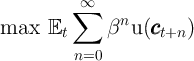
The economy consists of a continuum of households of mass one distributed on the unit interval, each of which maximizes expected discounted utility from consumption,
 |
for a CRRA utility function
u(∙) = ∙1-ρ∕(1-ρ).18
The household consumption functions {ct+n}n=0∞ satisfy:
 t = ptW, so that when
aggregate shocks are shut down the only state variable is (normalized) cash-on-hand
mt.19
t = ptW, so that when
aggregate shocks are shut down the only state variable is (normalized) cash-on-hand
mt.19
Households die with a constant probability D ≡ 1 - between
periods.20
Consequently, the effective discount factor is β
between
periods.20
Consequently, the effective discount factor is β (in (7)). The effective interest
rate is (ℸ + r)∕
(in (7)). The effective interest
rate is (ℸ + r)∕ , where ℸ = 1 - δ denotes the depreciation factor for capital
and r is the interest rate (which here is time-invariant and thus has no time
subscript).21
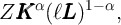
The production function is Cobb–Douglas:
, where ℸ = 1 - δ denotes the depreciation factor for capital
and r is the interest rate (which here is time-invariant and thus has no time
subscript).21
The production function is Cobb–Douglas:
 | (12) |
where Z is aggregate productivity,  is capital, ℓ is time worked per employee
and
is capital, ℓ is time worked per employee
and  is employment. The wage rate and the interest rate are equal to the
marginal product of labor and capital, respectively.
is employment. The wage rate and the interest rate are equal to the
marginal product of labor and capital, respectively.
As shown in (8)–(10), the evolution of household’s market resources mt can be broken up into three steps:
 |
 |

Solving maximization (7)–(11) gives the optimal consumption rule. A target wealth-to-permanent-income ratio exists if a death-modified version of Carroll (2011)’s ‘Growth Impatience Condition’ holds (see Appendix C of Carroll, Slacalek, and Tokuoka (2013) for derivation):
where R = ℸ + r, and Γ is labor productivity growth (the growth rate of permanent income).
| Description | Parameter | Value | Source |
| Representative agent model
| |||
| Time discount factor | β | 0.99 | JEDC (2010) |
| Coef of relative risk aversion | ρ | 1 | JEDC (2010) |
| Capital share | α | 0.36 | JEDC (2010) |
| Depreciation rate | δ | 0.025 | JEDC (2010) |
| Time worked per employee | ℓ | 1/0.9 | JEDC (2010) |
| Steady state
| |||
| Capital/(quarterly output) ratio |  ∕ ∕ | 10.26 | JEDC (2010) |
| Effective interest rate | r - δ | 0.01 | JEDC (2010) |
| Wage rate | W | 2.37 | JEDC (2010) |
| Heterogenous agents models
| |||
| Unempl insurance payment | μ | 0.15 | JEDC (2010) |
| Probability of death | D | 0.00625 | Yields 40-year working life |
| FBS income shocks
| |||
| Variance of log θt,i | σθ2 | 0.010 × 4 | Carroll (1992), |
| Carroll, Slacalek, and Tokuoka (2013) | |||
| Variance of log ψt,i | σψ2 | 0.010∕4 | Carroll (1992), |
| DeBacker et al. (2013), | |||
| Carroll, Slacalek, and Tokuoka (2013) | |||
| Unemployment rate | u | 0.07 | Mean in JEDC (2010) |
| Variance of log Ξt | σΞ2 | 0.00001 | Authors’ calculations |
| Variance of log Ψt | σΨ2 | 0.00004 | Authors’ calculations |
| KS income shocks
| |||
| Aggregate shock to productivity | △Z | 0.01 | Krusell and Smith (1998) |
| Unemployment (good state) | ug | 0.04 | Krusell and Smith (1998) |
| Unemployment (bad state) | ub | 0.10 | Krusell and Smith (1998) |
| Aggregate transition probability | 0.125 | Krusell and Smith (1998) | |
Notes: The models are calibrated at the quarterly frequency, and the steady state values are calculated on a quarterly basis.
We calibrate the standard elements of the model using the parameter values used for the papers in the special issue of the Journal of Economic Dynamics and Control (2010) devoted to comparing solution methods for the KS model (the parameters are reproduced for convenience in Table 2). The model is calibrated at the quarterly frequency.
We calibrate the FBS income process as follows. The variances of idiosyncratic components are taken from Carroll (1992) because those numbers are representative of the large subsequent empirical literature all the way through the new paper by DeBacker, Heim, Panousi, Ramnath, and Vidangos (2013) whose point estimate of the variance of the permanent shock almost exactly matches the calibration in Carroll (1992).22
The variances of the aggregate income process were estimated as follows, using
U.S. NIPA labor income, constructed as wages and salaries plus transfers
minus personal contributions for social insurance. We first calibrate the
signal-to-noise ratio ς ≡ σΨ2 σΞ2 so that the first autocorrelation of the
process, generated using the logged versions of equations (5)–(6), is
0.96.23 ,24
Differencing equation (5) and expressing the second moments yields
σΞ2 so that the first autocorrelation of the
process, generated using the logged versions of equations (5)–(6), is
0.96.23 ,24
Differencing equation (5) and expressing the second moments yields
 Δ log
Δ log  t
t and ς we identify σΞ2 = var
 Δ log
Δ log  t
t
 (ς + 2)
and σΨ2 = ςσΞ2. The strategy yields the following estimates: ς = 4,
σΨ2 = 4.29 × 10⁻⁵ and σΞ2 = 1.07 × 10⁻⁵ (given in Table 2).
(ς + 2)
and σΨ2 = ςσΞ2. The strategy yields the following estimates: ς = 4,
σΨ2 = 4.29 × 10⁻⁵ and σΞ2 = 1.07 × 10⁻⁵ (given in Table 2).
This parametrization of the aggregate income process yields income dynamics that match the same aggregate statstics that are matched by standard exercises in the real business cycle literature including Jermann (1998), Boldrin, Christiano, and Fisher (2001), and Chari, Kehoe, and McGrattan (2005). It also fits well the broad conclusion of the large literature on unit roots of the 1980s, which found that it is virtually impossible to reject the existence of a permanent component in aggregate income series (see Stock (1986) for a review).
To finish calibrating the model, we assume (for now) that all households have an
identical time preference factor β =  (corresponding to a point distribution of
β) and henceforth call this specification the ‘β-Point’ model. With no aggregate
uncertainty, we follow the procedure of the papers in the JEDC volume
by backing out the value of
(corresponding to a point distribution of
β) and henceforth call this specification the ‘β-Point’ model. With no aggregate
uncertainty, we follow the procedure of the papers in the JEDC volume
by backing out the value of  for which the steady-state value of the
capital-to-output ratio (
for which the steady-state value of the
capital-to-output ratio ( ∕
∕ ) matches the value that characterized the
steady-state of the perfect foresight version of the model;
) matches the value that characterized the
steady-state of the perfect foresight version of the model;  turns out to be
0.9899 (at a quarterly rate).
turns out to be
0.9899 (at a quarterly rate).
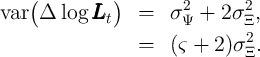
Carroll, Slacalek, and Tokuoka (2013) show that the β-Point model matches the empirical wealth distribution substantially better than the version of the Krusell and Smith (1998) model analyzed in the Journal of Economic Dynamics and Control (2010) volume, which we call ‘KS-JEDC.’25 For example, while the top 1 percent households living in the KS-JEDC model own only 3 percent of total wealth,26 those living in the β-Point are much richer, holding roughly 10 percent of total wealth. This improvement is driven by the presence of the permanent shock to income, which generates heterogeneity in the level of wealth because, while all households have the same target wealth/permanent income ratio, the equilibrium dispersion in the level of permanent income leads to a corresponding equilibrium dispersion in the level of wealth.
Figure 1 illustrates these results by plotting the wealth Lorenz curves implied by alternative models. Introducing the FBS shocks into the framework makes the Lorenz curve for the KS-JEDC model move roughly one third of the distance toward the data from the 2004 Survey of Consumer Finances,27 to the dashed curve labeled β-Point.
However, the wealth heterogeneity in the β-Point model essentially just replicates heterogeneity in permanent income (which accounts for most of the heterogeneity in total income); for example the Gini coefficient for permanent income measured in the Survey of Consumer Finances of roughly 0.5 is similar to that for wealth generated in the β-Point model. Since the empirical distribution of wealth (which has the Gini coefficient of around 0.8) is considerably more unequal than the distribution of income (or permanent income), the setup only captures part of the wealth heterogeneity in the data, especially at the top.
Because we want a modeling framework that matches the fact that wealth inequality substantially exceeds income inequality, we need to introduce an additional source of heterogeneity (beyond heterogeneity in permanent and transitory income). We accomplish this by introducing heterogeneity in impatience. Each household is now assumed to have an idiosyncratic (but fixed) time preference factor. We think of this assumption as reflecting not only actual variation in pure rates of time preference across people, but also as reflecting other differences (in age, income growth expectations, investment opportunities, tax schedules, risk aversion, and other variables) that are not explicitly incorporated into the model.
To be more concrete, take the example of age. A robust pattern in most countries is that income grows much faster for young people than for older people. Our “death-modified growth impatience condition” (13) captures the intuition that people facing faster income growth tend to act, financially, in a more ‘impatient’ fashion than those facing lower growth. So we should expect young people to have lower target wealth-to-income ratios than older people. Thus, what we are capturing by allowing heterogeneity in time preference factors is probably also some portion of the difference in behavior that (in truth) reflects differences in age instead of in pure time preference factors. Some of what we achieve by allowing heterogeneity in β could alternatively be introduced into the model if we had a more complex specification of the life cycle that allowed for different income growth rates for households of different ages.28
One way of gauging a model’s predictions for wealth inequality is to ask how well it is able to match the proportion of total net worth held by the wealthiest 20, 40, 60, and 80 percent of the population. We follow other papers (in particular Castaneda, Diaz-Gimenez, and Rios-Rull (2003)) in matching these statistics.29
Our specific approach is to replace the assumption that all households
have the same time preference factor with an assumption that, for some
dispersion ∇, time preference factors are distributed uniformly in the
population between  -∇ and
  + ∇ (for this reason, the model is referred
to as the ‘β-Dist’ model). Then, using simulations, we search for the
values of
+ ∇ (for this reason, the model is referred
to as the ‘β-Dist’ model). Then, using simulations, we search for the
values of  and ∇ for which the model best matches the fraction of net
worth held by the top 20, 40, 60, and 80 percent of the population,
while at the same time matching the aggregate capital-to-output ratio
from the perfect foresight model. Specifically, defining wi and ωi as the
proportion of total aggregate net worth held by the top i percent in our
model and in the data, respectively, we solve the following minimization
problem:
and ∇ for which the model best matches the fraction of net
worth held by the top 20, 40, 60, and 80 percent of the population,
while at the same time matching the aggregate capital-to-output ratio
from the perfect foresight model. Specifically, defining wi and ωi as the
proportion of total aggregate net worth held by the top i percent in our
model and in the data, respectively, we solve the following minimization
problem:
 | (14) |
subject to the constraint that the aggregate wealth (net worth)-to-output ratio in the
model matches the aggregate capital-to-output ratio from the perfect foresight model
( PF∕
PF∕ PF):30
 ,∇} = {0.9876, 0.0060}, so that
the discount factors are evenly spread roughly between 0.98 and
0.99.31
,∇} = {0.9876, 0.0060}, so that
the discount factors are evenly spread roughly between 0.98 and
0.99.31
The introduction of even such a relatively modest amount of time preference heterogeneity sharply improves the model’s fit to the targeted proportions of wealth holdings, bringing it reasonably in line with the data (Figure 1). The ability of the model to match the targeted moments does not, of course, constitute a formal test, except in the loose sense that a model with such strong structure might have been unable to get nearly so close to four target wealth points with only one free parameter.32 But the model also sharply improves the fit to locations in the wealth distribution that were not explicitly targeted; for example, the net worth shares of the top 10 percent and the top 1 percent are also included in the table, and the model performs reasonably well in matching them.
Of course, Krusell and Smith (1998) were well aware that their baseline model provides a poor match to the wealth distribution. In response, they examined whether inclusion of a form of discount rate heterogeneity could improve the model’s match to the data. Specifically, they assumed that the discount factor takes one of the three values (0.9858, 0.9894, and 0.9930), and that agents anticipate that their discount factor might change between these values according to a Markov process. As they showed, the model with this simple form of heterogeneity did improve the model’s ability to match the wealth holdings of the top percentiles. Indeed, unpublished results kindly provided by the authors show their model of heterogeneity went a bit too far: it concentrated almost all of the net worth in the top 20 percent of the population. By comparison, our model β-Dist does a notably better job matching the data across the entire span of wealth percentiles.
The reader might wonder why we do not simply adopt the KS specification of heterogeneity in time preference factors, rather than introducing our own novel (though simple) form of heterogeneity. The principal answer is that our purpose here is to define a method of explicitly matching the model to the data via statistical estimation of a parameter of the distribution of heterogeneity, letting the data speak flexibly to the question of the extent of the heterogeneity required to match model to data. Krusell and Smith were not estimating a distribution in this manner; estimation of their framework would have required searching for more than one parameter, and possibly as many as three of four. Indeed, had they intended to estimate parameters, they might have chosen a method more like ours. A second point is that, having introduced finite horizons in order to yield an ergodic distribution of permanent income, it would be peculiar to layer on top of the stochastic death probability a stochastic probability of changing one’s time preference factor within the lifetime; Krusell and Smith motivated their differing time preference factors as reflecting different preferences of alternating generations of a dynasty, but with our finite horizons assumption we have eliminated the dynastic interpretation of the model. Having said all of this, the common point across the two papers is that a key requirement to make the model fit the wealth data is a form of heterogeneity that leads different households to have different target levels of wealth.
Having constructed a model with a realistic household income process which is able to reproduce steady-state wealth heterogeneity in the data, we now turn on aggregate shocks and investigate the model’s implications about relevant macroeconomic questions. In particular, we ask whether a model that manages to match the distribution of wealth has similar, or different, implications from the KS-JEDC or representative agent models for the reaction of aggregate consumption to an economic ‘stimulus’ payment.
Specifically, we pose the question as follows. The economy has been in its steady-state equilibrium leading up to date t. Before the consumption decision is made in that period, the government announces the following plan: effective immediately, every household in the economy will receive a one-off ‘stimulus check’ worth some modest amount $x (financed by a tax on unborn future generations).33 Our question is: By how much will aggregate consumption increase?
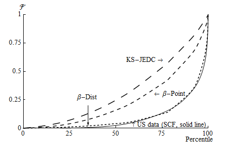
In theory, the distribution of wealth across recipients of the stimulus checks has important implications for aggregate MPC out of transitory shocks to income. To see why, the solid line of Figure 2 plots our β-Point model’s individual consumption function using the FBS aggregate income process, with the horizontal axis being cash on hand normalized by the level of (quarterly) permanent income. Because the households with less normalized cash have higher MPCs, the average MPC is higher when a larger fraction of households has less (normalized) cash on hand.
There are many more households with little wealth in our β-Point model than in the KS-JEDC model, as illustrated by comparison of the short-dashing and the long-dashing lines in Figure 1. The greater concentration of wealth at the bottom in the β-Point model, which mirrors the data (see the histogram in Figure 2), should produce a higher average MPC, given the concave consumption function.
Indeed, the average MPC out of the transitory income (‘stimulus check’) in our β-Point model is 0.1 in annual terms (second column of Table 3),34 about double the value in the KS-JEDC model (0.05) (first column of the table) or the perfect foresight partial equilibrium model with paramters matching our baseline calibration (0.04). Our β-Dist model (third column of the table) produces an even higher average MPC (0.23), since in the β-Dist model there are more households who possess less wealth, are more impatient, and have higher MPCs (Figure 1 and dashed lines in Figure 2). However, this is still at best only at the lower bound of empirical MPC estimates, which are typically between 0.2–0.6 or even higher (see Table 1).
| Krusell–Smith (KS) | Friedman/Buffer Stock (FBS)
| |||||
| Aggregate Process | Aggregate Process
| |||||
| Model | KS-JEDC | β-Point | β-Dist | β-Dist | β-Dist | β-Dist
|
| Our Solution | ||||||
| Wealth Measure | Net | Net | Liquid Financial | Net | Liquid Financial
| |
| Worth | Worth | and Retirement | Worth | and Retirement | ||
| Assets | Assets
| |||||
| Overall average | 0.05 | 0.10 | 0.23 | 0.43 | 0.20 | 0.42 |
| By wealth/permanent income ratio | ||||||
| Top 1% | 0.04 | 0.06 | 0.05 | 0.12 | 0.05 | 0.12 |
| Top 10% | 0.04 | 0.06 | 0.06 | 0.12 | 0.06 | 0.12 |
| Top 20% | 0.04 | 0.06 | 0.06 | 0.13 | 0.06 | 0.13 |
| Top 40% | 0.04 | 0.06 | 0.08 | 0.20 | 0.06 | 0.17 |
| Top 50% | 0.05 | 0.07 | 0.09 | 0.23 | 0.06 | 0.22 |
| Top 60% | 0.04 | 0.07 | 0.12 | 0.28 | 0.09 | 0.24 |
| Bottom 50% | 0.05 | 0.13 | 0.35 | 0.59 | 0.32 | 0.58 |
| By income | ||||||
| Top 1% | 0.05 | 0.08 | 0.12 | 0.17 | 0.16 | 0.36 |
| Top 10% | 0.05 | 0.08 | 0.15 | 0.27 | 0.17 | 0.36 |
| Top 20% | 0.05 | 0.09 | 0.16 | 0.31 | 0.17 | 0.37 |
| Top 40% | 0.05 | 0.10 | 0.18 | 0.34 | 0.19 | 0.38 |
| Top 50% | 0.05 | 0.11 | 0.19 | 0.35 | 0.18 | 0.39 |
| Top 60% | 0.05 | 0.10 | 0.19 | 0.37 | 0.20 | 0.39 |
| Bottom 50% | 0.05 | 0.09 | 0.27 | 0.50 | 0.22 | 0.45 |
| By employment status | ||||||
| Employed | 0.05 | 0.09 | 0.20 | 0.39 | 0.19 | 0.39 |
| Unemployed | 0.06 | 0.23 | 0.54 | 0.80 | 0.41 | 0.73 |
| Time preference parameters‡ | ||||||
 | 0.9899 | 0.9848 | 0.9570 | 0.9876 | 0.9636 | |
| ∇ | 0.0094 | 0.0210 | 0.0060 | 0.0133 | ||
Notes: Annual MPC is calculated by 1 - (1-quarterly MPC)4. ‡: Discount factors are uniformly distributed
over the interval [ -∇,
-∇, + ∇].
+ ∇].
Comparison of columns 3 and 5 of Table 3 makes it clear that for the purpose of backing out the aggregate MPC, the particular form of the aggregate income process is not essential; both in qualitative and in quantitative terms the aggregate MPC and its breakdowns for the KS and the FBS aggregate income specification lie close to each other. This finding is in line with a large literature sparked by Lucas (1985) about the modest welfare cost of the aggregate fluctuations associated with business cycles and with the calibration of Table 2, in which variance of aggregate shocks is roughly two orders of magnitude smaller than variance of idiosyncratic shocks. (Of course, if one consequence of business cycles is to increase the magnitude of idiosyncratic shocks, as suggested for example by McKay and Papp (2011), Guvenen, Ozkan, and Song (2012) and Blundell, Low, and Preston (2013), the costs of business cycles could be much larger than in traditional calculations that examine only the consequences of aggregate shocks.)
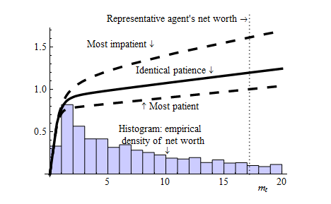
Thus far, we have been using total household net worth as our measure of wealth. Implicitly, this assumes that all of the household’s debt and asset positions are perfectly liquid and that, say, a household with home equity of $50,000 and bank balances of $2,000 (and no other balance sheet items) will behave in every respect similarly to a household with home equity of $10,000 and bank balances of $42,000. This seems implausible. The home equity is more illiquid (tapping it requires, at the very least, obtaining a home equity line of credit, with the attendant inconvenience and expense of appraisal of the house and some paperwork).
Otsuka (2004) formally analyzes the optimization problem of a consumer with a FBS income process who can invest in an illiquid but higher-return asset (think housing), or a liquid but lower-return asset (cash), and shows, unsurprisingly, that the annual marginal propensity to consume out of shocks to liquid assets is higher than the MPC out of shocks to illiquid assets. Her results would presumably be even stronger if she had permitted households to hold much of their wealth in illiquid forms (housing, pension savings), for example, as a mechanism to overcome self-control problems (see Laibson (1997) and many others).35
These considerations suggest that it may be more plausible, for purposes of extracting predictions about the MPC out of stimulus checks, to focus on matching the distribution of liquid financial and retirement assets across households. The inclusion of retirement assets is arguable, but a case for inclusion can be made because in the U.S. retirement assets such as IRA’s and 401(k)’s can be liquidated under a fairly clear rule (e.g., a penalty of 10 percent of the balance liquidated).
| Net Worth | Liquid Financial
| |
| and Retirement Assets
| ||
| Top 1% | 33.9 | 34.6 |
| Top 10% | 69.7 | 75.3 |
| Top 20% | 82.9 | 88.3 |
| Top 40% | 94.7 | 97.5 |
| Top 60% | 99.0 | 99.6 |
| Top 80% | 100.2 | 100.0 |
Notes: The data source is the 2004 Survey of Consumer Finances.
When we ask the model to estimate the time preference factors that allow it to
best match the distribution of liquid financial and retirement assets (instead of net
worth),36
estimated parameter values are { ,∇} = {0.9570, 0.0210} under the KS
aggregate income process and the average MPC is 0.44 (fourth column of the
table), which lies at the middle of the range typically reported in the literature
(see Table 1), and is considerably higher than when we match the distribution of
net worth. This reflects the fact that matching the more skewed distribution of
liquid financial and retirement assets than that of net worth (Table 4 and
Figure 3) requires a wider distribution of the time preference factors, ranging
between 0.94 and 0.975, which produces even more households with little
wealth.37
The estimated distribution of discount factors lies below that obtained by
matching net worth and is considerably more dispersed because of substantially
lower median and more unevenly distributed liquid financial and retirement
assets (compared to net worth).
,∇} = {0.9570, 0.0210} under the KS
aggregate income process and the average MPC is 0.44 (fourth column of the
table), which lies at the middle of the range typically reported in the literature
(see Table 1), and is considerably higher than when we match the distribution of
net worth. This reflects the fact that matching the more skewed distribution of
liquid financial and retirement assets than that of net worth (Table 4 and
Figure 3) requires a wider distribution of the time preference factors, ranging
between 0.94 and 0.975, which produces even more households with little
wealth.37
The estimated distribution of discount factors lies below that obtained by
matching net worth and is considerably more dispersed because of substantially
lower median and more unevenly distributed liquid financial and retirement
assets (compared to net worth).
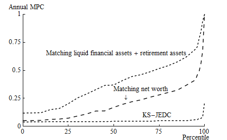
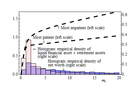
Figure 4 shows the cumulative distribution functions of MPCs for the KS-JEDC model and the β-Dist models (under the KS aggregate income shocks) estimated to match, first, the empirical distribution of net worth and, alternatively, of liquid financial and retirement assets.38 The figure illustrates that the MPCs for KS-JEDC model are concentrated tightly around 0.05, which sharply contrasts with the results for the β-Dist models. Because the latter two models match the empirical wealth distribution, they imply that a substantial fraction of consumers has very little wealth.
Table 3 illustrates the distribution of MPCs by wealth, income, and employment status. In contrast to the KS-JEDC model, the β-Point and in particular β-Dist models generate a wide distribution of marginal propensities. Given the considerable concavity of the theoretical consumption function in the relevant region, these results indicate that the aggregate response to a stimulus program will depend greatly upon which households receive the stimulus payments. Furthermore, unlike the results from the baseline KS-JEDC model or from a representative agent model, the results from these simulations are easily consistent with the empirical estimates of aggregate MPCs in Table 1 and the evidence that households with little liquid wealth and without high past income have high MPCs.39
Because our models include FBS or KS aggregate shocks, we can investigate how the economy’s average MPC and its distribution across households varies over the business cycle. Table 5 reports the results for the following experiments with the β-Dist models calibrated to the net worth distribution (and compares them to the baseline results from Table 3). For the model with KS aggregate shocks, in which recessions/expansions can be defined as bad/good realizations of the aggregate state:
For the model with FBS aggregate shocks, we consider large bad realizations of the aggregate shock:
| Model | Krusell–Smith (KS): β-Dist | Friedman/Buffer Stock (FBS): β-Dist
| ||||||
| Scenario | Entering | Large Bad Permanent | Large Bad Transitory
| |||||
| Baseline | Recession | Expansion | Recession | Baseline | Aggregate Shock | Aggregate Shock
| ||
| Overall average | 0.23 | 0.25 | 0.21 | 0.23 | 0.20 | 0.20 | 0.21 | |
| By wealth/permanent income ratio | ||||||||
| Top 1% | 0.05 | 0.05 | 0.05 | 0.05 | 0.05 | 0.05 | 0.05 | |
| Top 10% | 0.06 | 0.06 | 0.06 | 0.06 | 0.06 | 0.06 | 0.06 | |
| Top 20% | 0.06 | 0.06 | 0.06 | 0.06 | 0.06 | 0.06 | 0.06 | |
| Top 40% | 0.08 | 0.08 | 0.08 | 0.08 | 0.06 | 0.06 | 0.06 | |
| Top 50% | 0.09 | 0.10 | 0.09 | 0.09 | 0.06 | 0.06 | 0.09 | |
| Top 60% | 0.12 | 0.12 | 0.11 | 0.12 | 0.09 | 0.09 | 0.09 | |
| Bottom 50% | 0.35 | 0.38 | 0.32 | 0.35 | 0.32 | 0.32 | 0.32 | |
| By income | ||||||||
| Top 1% | 0.12 | 0.13 | 0.11 | 0.13 | 0.16 | 0.16 | 0.17 | |
| Top 10% | 0.15 | 0.16 | 0.15 | 0.16 | 0.17 | 0.17 | 0.17 | |
| Top 20% | 0.16 | 0.17 | 0.16 | 0.17 | 0.17 | 0.17 | 0.18 | |
| Top 40% | 0.18 | 0.19 | 0.18 | 0.18 | 0.19 | 0.19 | 0.19 | |
| Top 50% | 0.19 | 0.20 | 0.18 | 0.19 | 0.18 | 0.19 | 0.20 | |
| Top 60% | 0.19 | 0.20 | 0.19 | 0.20 | 0.20 | 0.20 | 0.20 | |
| Bottom 50% | 0.27 | 0.30 | 0.24 | 0.27 | 0.22 | 0.21 | 0.22 | |
| By employment status | ||||||||
| Employed | 0.20 | 0.20 | 0.20 | 0.20 | 0.19 | 0.19 | 0.19 | |
| Unemployed | 0.54 | 0.56 | 0.51 | 0.47 | 0.41 | 0.41 | 0.41 | |
Notes: Annual MPC is calculated by 1 - (1-quarterly MPC)4. The scenarios are calculated for the β-Dist models calibrated to the net worth distribution. For the KS aggregate shocks, the results are obtained by running the simulation over 1,000 periods, and the scenarios are defined as (i) ‘Recessions/Expansions’: bad/good realization of the aggregate state, 1 -△Z/1 + △Z; (ii) ‘Entering Recession’: bad realization of the aggregate state directly preceded by a good one: Zt = 1 -△Z for which Zt-1 = 1 + △Z. The ‘baseline’ KS results are reproduced from column 3 of Table 3. For the FBS aggregate shocks, the results are averages over 1,000 simulations, and the scenarios are defined as (i) ‘Large Bad Permanent Aggregate Shock’: bottom 1 percent of the distribution in the permanent aggregate shock; (ii) ‘Large Bad Transitory Aggregate Shock’: bottom 1 percent of the distribution in the transitory aggregate shock. The ‘baseline’ FBS results are reproduced from column 5 of Table 3.
In the KS setup, the aggregate MPC is countercyclical, ranging between 0.21 in expansions and 0.25 in recessions. The key reason for this business cycle variation lies in the fact that aggregate shocks are correlated with idiosyncratic shocks. The movements in the aggregate MPC are driven by the households at the bottom of the distributions of wealth and income, which are not adequately insured. MPCs for rich and employed households essentially do not change over the business cycle. The scenario ‘Entering Recession’ documents that the length of the recession matters, so that initially the MPCs remain close to the baseline values, and increase only slowly as recession persists.
In the FBS setup, the distribution of the MPC displays very little cyclical variation for both transitory and permanent aggregate shocks. This fact is caused because the precautionary behavior of households is driven essentially exclusively by idiosyncratic shocks, as these shocks are two orders of magnitude larger (in terms of variance) and because they are uncorrelated with aggregate shocks.
Of course, these results are obtained under the assumptions that the parameters and expectations in the models are constant, and that the wealth distribution is exogenous. These assumptions are likely counterfactual in events like the Great Recession, during which objects like expectations about the future income growth or the extent of uncertainty may well have changed.
As Figure 2 suggests, the aggregate MPC in our models is a result of an (inter-related) interaction between two objects: The distribution of wealth and the consumption function(s). During the Great Recession, the distribution of net worth has shifted very substantially downward. Specifically, Bricker, Kennickell, Moore, and Sabelhaus (2012) document that over the 2007–2010 period median net worth fell 38.8 percent (in real terms).40 Ceteris paribus, these dynamics resulted an increase in the aggregate MPC, as the fraction of wealth-poor, high-MPC households rose substantially.
It is also likely that the second object, the consumption function, changed as many of its determinants (such as the magnitude of income shocks41 ) have not remained unaffected by the recession. And, of course, once parameters are allowed to vary, one needs to address the question about how households form expectations about these parameters. These factors make it quite complex to investigate adequately the numerous interactions potentially relevant for the dynamics of the MPC over the business cycle. Consequently, we leave the questions about the extent of cyclicality of the MPC in more complicated settings for future research.
We have shown that a model with a realistic microeconomic income process and modest heterogeneity in time preference rates is able to match the observed degree of inequality in the wealth distribution. Because many households in our model accumulate very little wealth, the aggregate marginal propensity to consume out of transitory income implied by our model, roughly 0.2–0.4 depending on the measure of wealth we ask our model to target, is consistent with most of the large estimates of the MPC reported in the microeconomic literature. Indeed, some of the dispersion in MPC estimates from the microeconomic literature (where estimates range up to 0.75 or higher) might be explainable by the model’s implication that there is no such thing as “the” MPC – the aggregate response to a transitory income shock should depend on details of the recipients of that shock in ways that the existing literature may not have been sensitive to (or may not have been able to measure). If some of the experiments reported in the literature reflected shocks that were concentrated in different regions of the wealth distribution than other experiments, considerable variation in empirical MPCs would be an expected consequence of the differences in the experiments.
Additionally, our work provides researchers with an easier framework for solving, estimating, and simulating economies with heterogeneous agents and realistic income processes than has heretofore been available. Although benefiting from the important insights of Krusell and Smith (1998), our framework is faster and easier to solve than the KS model or many of its descendants, and thus can be used as a convenient building block for constructing micro-founded models for policy-relevant analysis.
AGARWAL, SUMIT, CHUNLIN LIU, AND NICHOLAS S. SOULELES (2007): “The Response of Consumer Spending and Debt to Tax Rebates – Evidence from Consumer Credit Data,” Journal of Political Economy, 115(6), 986–1019.
AGARWAL, SUMIT, AND WENLAN QUIAN (2013): “Consumption and Debt Response to Unanticipated Income Shocks: Evidence from a Natural Experiment in Singapore,” IRES working paper 18, National University of Singapore.
BLANCHARD, OLIVIER J. (1985): “Debt, Deficits, and Finite Horizons,” Journal of Political Economy, 93(2), 223–247.
BLUNDELL, RICHARD, HAMISH LOW, AND IAN PRESTON (2013): “Decomposing changes in income risk using consumption data,” Quantitative Economics, 4(1), 1–37.
BLUNDELL, RICHARD, LUIGI PISTAFERRI, AND IAN PRESTON (2008): “Consumption Inequality and Partial Insurance,” American Economic Review, 98(5), 1887–1921.
BLUNDELL, RICHARD, LUIGI PISTAFERRI, AND ITAY SAPORTA-EKSTEN (2012): “Consumption Inequality and Family Labor Supply,” NBER Working Papers 18445, National Bureau of Economic Research, Inc.
BOLDRIN, MICHELE, LAWRENCE J. CHRISTIANO, AND JONAS D. FISHER (2001): “Habit Persistence, Asset Returns and the Business Cycle,” American Economic Review, 91(1), 149–66.
BRICKER, JESSE, ARTHUR B. KENNICKELL, KEVIN B. MOORE, AND JOHN SABELHAUS (2012): “Changes in U.S. Family Finances from 2007 to 2010: Evidence from the Survey of Consumer Finances,” Federal Reserve Bulletin, 98(2), 1–80.
BRODA, CHRISTIAN, AND JONATHAN A. PARKER (2012): “The Economic Stimulus Payments of 2008 and the Aggregate Demand for Consumption,” mimeo, Northwestern University.
BROWNING, MARTIN, AND M. DOLORES COLLADO (2001): “The Response of Expenditures to Anticipated Income Changes: Panel Data Estimates,” American Economic Review, 91(3), 681–692.
CARROLL, CHRISTOPHER D. (1992): “The Buffer-Stock Theory of Saving: Some Macroeconomic Evidence,” Brookings Papers on Economic Activity, 1992(2), 61–156, http://www.econ2.jhu.edu/people/ccarroll/BufferStockBPEA.pdf.
__________ (2011): “Theoretical Foundations of Buffer Stock Saving,” Manuscript, Department of Economics, Johns Hopkins University, http://www.econ2.jhu.edu/people/ccarroll/papers/BufferStockTheory.
CARROLL, CHRISTOPHER D., JIRI SLACALEK, AND KIICHI TOKUOKA (2013): “Buffer-Stock Saving in a Krusell–Smith World,” mimeo, Johns Hopkins University.
CASTANEDA, ANA, JAVIER DIAZ-GIMENEZ, AND JOSE-VICTOR RIOS-RULL (2003): “Accounting for the U.S. Earnings and Wealth Inequality,” Journal of Political Economy, 111(4), 818–857.
CHARI, V. V., PATRICK J. KEHOE, AND ELLEN R. MCGRATTAN (2005): “A Critique of Structural VARs Using Real Business Cycle Theory,” working paper 631, Federal Reserve Bank of Minneapolis.
CORONADO, JULIA LYNN, JOSEPH P. LUPTON, AND LOUISE M. SHEINER (2005): “The Household Spending Response to the 2003 Tax Cut: Evidence from Survey Data,” FEDS discussion paper 32, Federal Reserve Board.
DEATON, ANGUS S. (1991): “Saving and Liquidity Constraints,” Econometrica, 59, 1221–1248.
__________ (1992): Understanding Consumption. Oxford University Press, New York.
DEBACKER, JASON, BRADLEY HEIM, VASIA PANOUSI, SHANTHI RAMNATH, AND IVAN VIDANGOS (2013): “Rising Inequality: Transitory or Permanent? New Evidence from a Panel of US Tax Returns,” mimeo.
DEN HAAN, WOUTER J., KENNETH L. JUDD, AND MICHEL JUILLARD (2010): “Computational Suite of Models with Heterogeneous Agents: Incomplete Markets and Aggregate Uncertainty,” Journal of Economic Dynamics and Control, 34(1), 1–3.
FRIEDMAN, MILTON A. (1957): A Theory of the Consumption Function. Princeton University Press.
GUVENEN, FATIH, SERDAR OZKAN, AND JAE SONG (2012): “The Nature of Countercyclical Income Risk,” Working Paper 18035, National Bureau of Economic Research.
HAUSMAN, JOSHUA K. (2012): “Fiscal Policy and Economic Recovery: The Case of the 1936 Veterans’ Bonus,” mimeo, University of California, Berkeley.
HSIEH, CHANG-TAI (2003): “Do Consumers React to Anticipated Income Changes? Evidence from the Alaska Permanent Fund,” American Economic Review, 93(1), 397–405.
JAPPELLI, TULLIO, AND LUIGI PISTAFERRI (2010): “The Consumption Response to Income Changes,” The Annual Review of Economics, 2, 479–506.
__________ (2013): “Fiscal Policy and MPC Heterogeneity,” discussion paper 9333, CEPR.
JERMANN, URBAN J. (1998): “Asset Pricing in Production Economies,” Journal of Monetary Economics, 41(2), 257–75.
JOHNSON, DAVID S., JONATHAN A. PARKER, AND NICHOLAS S. SOULELES (2006): “Household Expenditure and the Income Tax Rebates of 2001,” American Economic Review, 96(5), 1589–1610.
__________ (2009): “The Response of Consumer Spending to Rebates During an Expansion: Evidence from the 2003 Child Tax Credit,” working paper, The Wharton School.
JOURNAL OF ECONOMIC DYNAMICS AND CONTROL (2010): “Computational Suite of Models with Heterogeneous Agents: Incomplete Markets and Aggregate Uncertainty,” edited by Wouter J. Den Haan, Kenneth L. Judd, Michel Juillard, 34(1), 1–100.
KAPLAN, GREG (2012): “Inequality and the Life Cycle,” Quantitative Economics, 3(3), 471–525.
KAPLAN, GREG, AND GIOVANNI L. VIOLANTE (2011): “A Model of the Consumption Response to Fiscal Stimulus Payments,” NBER Working Paper Number W17338.
KEYNES, JOHN MAYNARD (1936): The General Theory of Employment, Interest, and Money. Harcourt, Brace.
KREINER, CLAUS THUSTRUP, DAVID DREYER LASSEN, AND SØREN LETH-PETERSEN (2012): “Heterogeneous Responses and Aggregate Impact of the 2001 Income Tax Rebates,” discussion paper 9161, CEPR.
KRUSELL, PER, AND ANTHONY A. SMITH (1998): “Income and Wealth Heterogeneity in the Macroeconomy,” Journal of Political Economy, 106(5), 867–896.
LAIBSON, DAVID (1997): “Golden Eggs and Hyperbolic Discounting,” Quarterly Journal of Economics, CXII(2), 443–477.
LOW, HAMISH, COSTAS MEGHIR, AND LUIGI PISTAFERRI (2010): “Wage Risk and Employment Over the Life Cycle,” American Economic Review, 100(4), 1432–1467.
LUCAS, ROBERT E. (1985): Models of Business Cycles, Yrjo Jahnsson Lectures. Basil Blackwell, Oxford.
LUSARDI, ANNAMARIA (1996): “Permanent Income, Current Income, and Consumption: Evidence from Two Panel Data Sets,” Journal of Business and Economic Statistics, 14(1), 81–90.
MCKAY, ALISDAIR, AND TAMAS PAPP (2011): “Accounting for Idiosyncratic Wage Risk Over the Business Cycle,” working paper 28, Boston University.
MISRA, KANISHA, AND PAOLO SURICO (2011): “Heterogeneous Responses and Aggregate Impact of the 2001 Income Tax Rebates,” discussion paper 8306, CEPR.
MOFFITT, ROBERT, AND PETER GOTTSCHALK (2011): “Trends in the Covariance Structure of Earnings in the U.S.: 1969–1987,” Journal of Economic Inequality, 9, 439–459, doi: 10.1007/s10888-010-9154-z.
OTSUKA, MISUZU (2004): “Household Portfolio Choice with Illiquid Assets,” PhD dissertation, Johns Hopkins University.
PARKER, JONATHAN (1999): “The Reaction of Household Consumption to Predictable Changes in Social Security Taxes,” American Economic Review, Vol 89(4), 959–73.
PARKER, JONATHAN A., NICHOLAS S. SOULELES, DAVID S. JOHNSON, AND ROBERT MCCLELLAND (2011): “Consumer Spending and the Economic Stimulus Payments of 2008,” NBER Working Paper Number W16684.
PISTAFERRI, LUIGI, AND ITAY SAPORTA-EKSTEN (2012): “Changes in the Income Distribution and Aggregate Consumption,” working paper 11, Ministry of Economy and Finance, Italy.
SAHM, CLAUDIA R., MATTHEW D. SHAPIRO, AND JOEL B. SLEMROD (2010): “Household Response to the 2008 Tax Rebate: Survey Evidence and Aggregate Implications,” Tax Policy and the Economy, 24, 69–110.
SHAPIRO, MATTHEW D., AND JOEL SLEMROD (2003): “Consumer Response to Tax Rebates,” American Economic Review, 93(1), 381–396.
__________ (2009): “Did the 2008 Tax Rebates Stimulate Spending?,” Manuscript, University of Michigan, http://www-personal.umich.edu/~shapiro/papers/Rebate2008-2008-12-27-assa-draft.pdf.
SOULELES, NICHOLAS S. (1999): “The Response of Household Consumption to Income Tax Refunds,” American Economic Review, 89(4), 947–958.
__________ (2002): “Consumer Response to the Reagan Tax Cuts,” Journal of Public Economics, 85, 99–120.
STOCK, JAMES H. (1986): “Unit roots, structural breaks and trends,” in Handbook of Econometrics, ed. by R. F. Engle, and D. McFadden, vol. 4 of Handbook of Econometrics, chap. 46, pp. 2739–2841. Elsevier.
STORESLETTEN, KJETIL, CHRIS I. TELMER, AND AMIR YARON (2004): “Consumption and Risk Sharing Over the Life Cycle,” Journal of Monetary Economics, 51(3), 609–633.
TOPEL, ROBERT H. (1991): “Specific Capital, Mobility and Wages: Wages Rise with Job Seniority,” Journal of Political Economy, 99, 145–176.
ZELDES, STEPHEN P. (1989): “Optimal Consumption with Stochastic Income: Deviations from Certainty Equivalence,” Quarterly Journal of Economics, 104(2), 275–298.


![[ ]
1- ρ
v(mt ) = macx u (ct) + β//D Et ψt+1 v(mt+1 ) (7)
t
s.t.
a = m - c , (8)
t t t
kt+1 = at∕(//D ψt+1 ), (9)
mt+1 = (ℸ + r)kt+1 + ξt+1, (10)
at ≥ 0, (11)](cstMPC10x.png)
![1∕ρ - 1
(R-β-)---E-[ψ---]//D- < 1, (13)
Γ](cstMPC22x.png)