^©May 9, 2008, Christopher Carroll qModel

This handout presents a discrete-time version of the Abel (1981)-Hayashi (1982) marginal ϙ model of investment.

1 Definitions

To simplify the algebra and intuition, we assume that a unit of investment purchased in period t does not become productive until time t + 1, so that the price paid in period t reflects the present discounted value of the period-t + 1 price of capital.¹ Adjustment costs are priced the same way.^{2 ,3}

kt	-	Firm’s capital stock at the beginning of period t
f(k)	-	Gross output excluding investment and adjustment costs
(1 - η)	-	Tax rate on corporate earnings
η	-	1 - (1 - η) = Portion of earnings untaxed
πt = f(kt)η	-	After tax revenues
it	-	Investment in period t (affects capital stock in period t + 1)
jt = j(it,kt)	-	AdJustment costs incurred in period t; smooth and convex
β = R-1	-	Discount factor for future profits (inverse of interest factor)
	-	Investment tax credit (ITC)
ζ	-	= 1 - = Cost of investment after ITC
pt	-	Price of one unit of investment
t = ζpt	-	Effective after-tax price of investment expenditures
xt = (it + jt) t+1β	-	Total after-tax period-t spending on investment (described above)
δ	-	Depreciation rate
ℸ	-	Depreciation factor = (1 - δ)
ω	-	Adjustment cost parameter

2 The Problem

The ϙ model assumes that firms want to maximize the net profits payable to shareholders, definable as the present discounted value of after-tax revenues after subtracting off costs of investment. Formally, the firm’s goal is

Next period’s capital is what remains of this period’s capital after depreciation, plus current investment,⁴

If capital markets are efficient, e_t will also be the stock market value of the profit-maximizing firm because it is precisely the amount a rational investor will be willing to pay if that investor cares only about discounted after-tax income derived from owning the firm.

The Bellman equation for the firm’s value can be derived (for = t + 1) from

So the PDV of the marginal cost (after tax, including adjustment costs) of an additional unit of investment should match the discounted expected marginal value of the resulting extra capital.

Recalling that π_t = ηf(k_t), the Envelope theorem for this problem can be used on either (4) or (5):

We now specify a convex (quadratic) adjustment cost function as

To begin interpreting this equation, consider first the case where the costs of adjustment are zero, ω = 0. In this case jⁱ = j^k = 0 and the Euler equation reduces to

Simplifying further, suppose that capital prices are constant at p = 1 and the ITC is unchanging so that the after-tax price of capital is constant at . Then since 1 + r + δ ≈ 1∕βℸ, the equation becomes

This says that the cost of buying one unit of capital, , is equal to the opportunity cost in lost interest plus the depreciation, (r + δ), which must match the (after-tax) payoff from ownership of that capital. Notice that this corresponds exactly to the formula for the equilibrium cost of capital in the HallJorgenson model: In the presence of an investment tax credit at rate , the after-tax price of capital is = ζ, and the firm will adjust its holdings of capital until

Now define λ_t ≡ e_t^k as the marginal value to the firm of ownership of one more unit of capital at the beginning of period t; using this definition the envelope condition can be written

This equation can best be understood as an arbitrage equation for the share price of the company if capital markets are efficient.⁶ The first term on the RHS rλ_t is the flow of income that would be obtained from putting the value of an extra unit of capital in the bank. The term in brackets [] is the flow value of having an extra unit of capital inside the firm: Extra revenues are measured by the first term, the second term accounts for the effect of the extra capital on costs of adjustment, and the final term reflects the cost to the firm of the extra depreciation that results from having more capital.

Think first about the 𝔼_tΔλ_t+1 = 0 case, in which the firm’s value, share price, and size will be unchanging because the marginal value of capital inside the firm is equal to the opportunity cost of employing that capital outside the firm (leaving it in the bank). If these two options yield equivalent returns, it is because the firm is already the ‘right’ size and should be neither growing nor shrinking.

Now consider the case where 𝔼_tΔλ_t+1 < 0, because

This says that an extra unit of capital is more valuable inside the firm than outside it, which means that 1) λ_t is above its steady-state value; 2) the firm will have positive net investment; and 3) the firm’s share value will be falling over time (because the level of its share value today is high, reflecting the fact that the high marginal valuation of the firm’s future investment has already been incorporated into λ_t). (The case with rising share prices is symmetric.)

Now define ‘marginal ϙ’ as the value of an additional unit of capital inside the firm divided by the after-tax price of an additional unit of capital,

The investment first order condition (6) implies

• At a value of ϙ_t+1 = 1, investment takes place at a rate exactly equal to the depreciation rate ((1) = 0)
• The investment ratio ι_t is monotonically increasing in ϙ_t+1 (^′(ϙ_t+1) > 0)
• The strength with which ι_t is related to ϙ_t+1 depends on the magnitude of adjustment costs (d|_t|∕dω < 0)

3 Phase Diagrams

3.1 Dynamics of k

The capital accumulation equation can be rewritten as

3.2 Dynamics of Δϙ

To construct a phase diagram involving ϙ, we need to transform our equation (33) for the dynamics of λ into an equation for the dynamics of ϙ. As a preliminary, define the proportional change in the after-tax price of capital as

Recalling that _t+1 = Δ _t+1 + _t, dividing both sides of (33) by _t yields

Now assuming that Δϙ_t+1, ∇ _t+1, r, and j_t^k are all ‘small’ so that their interactions are approximately 0, we have

Simplifying further, if the pretax price of capital is unchanging p_t+1 = p_t and δ = 0, (45) becomes

3.3 Results

Figure 1 presents two versions of the phase diagram, one for k and λ and one for k and ϙ.

For most purposes, ϙ diagram is simpler, because our facts about the function imply that the Δk_t+1 = 0 locus is always a horizontal line at ϙ = 1. This is because ϙ = 1 always corresponds to the circumstance in which the value of a unit of capital inside the firm, λ, matches the after-tax cost of a unit of capital, , so ϙ = 1 is the only value of ϙ at which the firm does not wish to change size (Δk_t+1 = 0).

The slope of the 𝔼[Δϙ_t+1] locus is easiest to think about near the steady state value of k where we can approximate j_t^k ≈ 0. Pick a point on the 𝔼[Δϙ_t+1] = 0 locus. Now consider a value of ϙ that is slightly larger. From (46), at the initial value of k we would have 𝔼[Δϙ_t+1] > 0. Thus, the value of k corresponding to 𝔼[Δϙ_t+1] = 0 must be one that balances the higher ϙ by a higher value of f^k, which is to say a lower value of k. This means that higher ϙ will be associated with lower k so that the locus is downward-sloping.

For appropriate choices of parameter values the problem satisfies the usual conditions for saddle point stability and will therefore have a saddle path solution, as depicted in the diagram.

The λ diagram is virtually indistinguishable from the ϙ diagram; the only difference is that the Δk_t+1 locus is located at the point λ = (i.e. the marginal value of investment is equal to the price of a unit of investment). The distinction between the diagrams reflects the fact that an increase in the investment tax credit will result in a rise in the steady-state value of k which implies a fall in the pretax marginal product of capital.

4 Dynamics

4.1 Steady State

The key to understanding the model’s dynamics is understanding the steady state toward which it is heading, then understanding how it gets there.

The key to the steady state, in turn, is that the capital stock will eventually be able to reach a point where j^k = jⁱ = 0.

4.2 A Positive Shock to Productivity

Suppose that the production function for the firm suddenly, permanently, and unexpectedly improves; specifically, suppose that leading up to period t the firm was in steady state, but in periods t + 1 and beyond the production function will be f_≥(k) = Ψf_<(k) for some Ψ > 1 where f_< and f_≥ indicate the production functions before and after the increase in productivity.

Note first that none of the tax terms has changed, and in the long run there is nothing to prevent the firm from adjusting its capital stock to the point consistent with the new level of productivity and then leaving it fixed there so that j^k = jⁱ = 0. Thus (46) implies that at the new steady state _≥ we will have r = ^-1f_≥^k(_≥) = Ψ^-1f_<^k(_≥) which implies _≥ > _<, since the steady state value of ϙ never changes: _≥ = _< = 1. That is, with higher productivity, the equilibrium capital stock is larger, but the equilibrium tax adjusted marginal product of capital is the same.

Obviously in order to get from an initial capital stock of _< to a larger equilibrium capital stock of _≥ the firm will need to engage in investment in excess of the depreciation rate, incurring costs of adjustment. In the absence of a change in the environment, expected costs of adjustment will always be declining toward zero, because the firm’s capital stock will always be moving toward its equilibrium value in which those costs are zero.

So we can tell the story as follows. Suppose that leading up to period t the firm was in its steady-state. When the productivity shock occurs, f^k jumps up. j_t^k had been zero (because the firm was at steady state), but now having more capital reduces the magnitude of future adjustment costs (the firm knows that its old steady-state capital stock is now too small, so it will have to be engaging in ι > 0 for a while), so j_t^k becomes negative. The combination ^-1f_t^k - j_t^kβ therefore becomes a larger positive number, so at the initial level of ϙ the RHS of (46) would imply 𝔼[Δϙ_t+1] less than zero, so the new 𝔼[Δϙ_t+1] = 0 locus must be higher (the equilibrating value of ϙ is higher). The saddle path is therefore also higher. So ϙ, and therefore ι, jump up instantly when the new higher level of productivity is revealed, corresponding also to an immediate increase in the firm’s share price (the marginal valuation of an additional unit of capital), since has not changed.

The phase diagrams with the saddle paths before and after the productivity increase together with the impulse response functions are plotted in figure 2.

4.3 A Permanent Tax Cut

Again starting from the steady state equilibrium, suppose unexpectedly and permanently decreases, which could happen because of a cut in corporate taxes or an increase in the ITC. (46) implies that in steady state

Dynamically, the story is as follows. (46) implies that following the tax change the 𝔼[Δϙ_t+1] = 0 locus must be higher because at any given ϙ the -f^k∕ term is a larger negative number, while at the initial k the j_t^k term is also now negative; so the 𝔼[Δϙ_t+1] = 0 locus shifts up.

In contrast to the case with a productivity shock, the equilibrium marginal product of capital will be lower than before. Arbitrage equalizes the after-tax marginal product of capital with the interest rate, but with a lower tax rate that will occur at a higher level of capital.

Notice that the qualitative story is the same whether the change in is due to a permanent reduction in the corporate tax rate (increase in η) or a permanent increase in the investment tax credit (reduction in ζ). In either case, ϙ and investment jump upward at time t and then gradually decline back toward their original steady-state levels.

There is, however, one interesting distinction between a decrease in due to a reduction in corporate taxes and a decrease caused by an increase in . Since λ = ζϙ, an increase in reduces ζ and therefore reduces the equilibrium value of λ, while a change in η has no effect on equilibrium λ. This reflects a subtle distinction. λ is the after-tax marginal value of extra capital, and the equilibrium in this model will occur at the point where that marginal value is equal to the marginal cost. Changing changes that marginal cost, so it changes the equilibrium after-tax marginal value. Changing η does not change the marginal cost of capital, so the equilibrium after-tax marginal value of capital is unchanged. The marginal product of capital is lower after a tax cut (equilibrium f^k is smaller), but that is exactly counterbalanced by the larger value of η so that ηf^k is unchanged in the long run by the change in η.

The phase diagrams with the saddle paths before and after the corporate tax reduction and the ITC increase together with the impulse response functions are respectively plotted in figures 3 and 4.

4.4 A Future Shock to Productivity

Now consider a circumstance where the firm knows that at some date in the future, t + n, the level of productivity will increase so that f_≥t+n = Ψf_<t+n for Ψ > 1.

The long run steady state is of course the same as in the example where the increase in productivity is immediately effective.

To determine the short run dynamics, notice several things. First, there can be no anticipated big jumps in the share price of the firm (the marginal productivity of capital inside the firm). Thus, if the productivity jump occurs in period t + n and the time periods are short enough, we must have

But because the equilibrium capital stock is larger, we know that j_≥t+n^k < 0 and will stay negative thereafter (asymptoting to zero from below). This reflects the fact that if you know you will need higher capital in the future, the most efficient way to minimize the cost of obtaining that capital is to gradually start building some of it even before you need it, rather than trying to do it all at once. Note further that before period t + n the model behaves according to the equations of motion defined by the problem under the < parameter values,⁷ while at t + n and after it behaves according to the new ≥ equations of motion.

Putting all this together, the story is as follows. Upon announcement of the productivity increase, λ jumps to the level such that, evolving exactly according to its < equations of motion, it will arrive in period t + n at a point exactly on the saddle path of the model corresponding to the ≥ equations of motion. Thereafter it will evolve toward the steady state, which will be at a higher level of capital than before, _≥ > _<, because the greater productivity justifies a higher equilibrium capital stock.

Thus, λ jumps up at time t, evolves to the northeast until time t + n, and thereafter asymptotes downward toward the same equilibrium value it had originally before the productivity change. Since has not changed, the dynamics of ϙ and ι are the same as those of λ.

4.5 A Future Tax Cut

Consider now the consequences if a tax cut is passed at date t that will become effective at date t + n > t.

Inspection of (46) might suggest that the effects of a future tax cut would be identical to the effects of a future increase in f^k, since the terms enter multiplicatively via ^-1f^k. And indeed, with respect to the dynamics of λ the two experiments are basically the same. And of course the steady-state value of ϙ is always equal to one.

During the transition, however, ϙ has interesting dynamics. From periods t to t + n - 1, taxes and the after-tax marginal product of capital do not change, and so the dynamics of ϙ are basically the same as those of λ. But between t + n- 1 and t + n, λ cannot jump but ^-1 does jump, which implies that ϙ must jump (so there is a predictable change in ϙ).

Dynamics of investment are determined by dynamics of ϙ, so the path of ι is: At t, a discrete jump up; between t and t + n, a gently rising path; between t + n- 1 and t + n, an upward jump; and after t + n, a path that asymptotes downward toward the steady state level of investment.

The steady-state effects on λ are of course determined by the same considerations as apply to the unanticipated tax cut, so they depend on whether the tax change is a drop in (1 -η) or an increase in .

References

Figure 1: Phase Diagrams

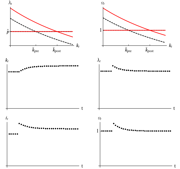
Figure 2: Increase in productivity: phase diagrams with saddle paths (dashed-black and continuous-red lines respectively pre and post the productivity increase) and impulse response functions

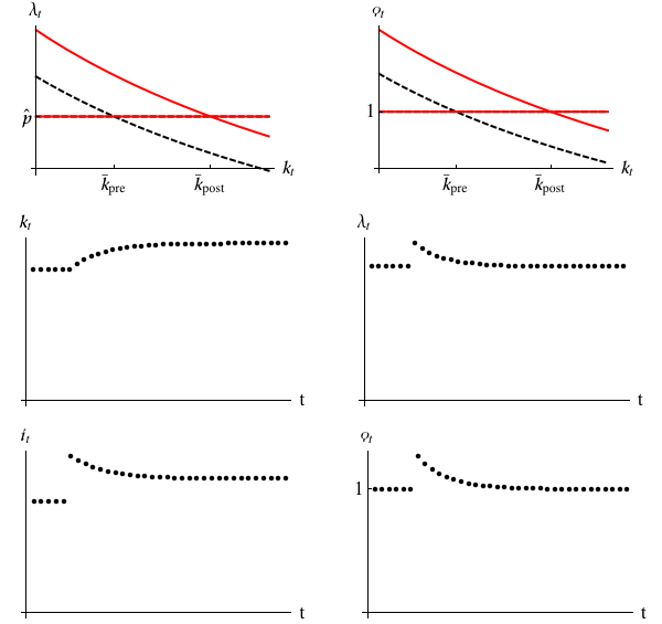
Figure 3: Corporate tax reduction: phase diagrams with saddle paths (dashed-black and continuous-red lines respectively pre and post the corporate tax reduction) and impulse response functions

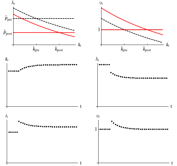
Figure 4: ITC increase: phase diagrams with saddle paths (dashed-black and continuous-red lines respectively pre and post the ITC increase) and impulse response functions

References

Abel, Andrew B. (1981): “A Dynamic Model of
Investment and Capacity Utilization,” Quarterly Journal of
Economics, 96(3), 379–403.
Hayashi, Fumio (1982): “Tobin’s Marginal Q and Average
Q: A Neoclassical Interpretation,” Econometrica, 50(1),