^©April 15, 2008, Christopher Carroll DecentralizingRCK

This handout shows that under certain very special conditions the behavior of an economy composed of distinct individual households will replicate the social planner’s solution to the Ramsey/Cass-Koopmans model.

1 The Consumer’s Problem

Consider first the problem of an individual infinitely lived consumer indexed by i who has some predetermined set of expectations for how the aggregate interest rate r_t and wage rate w_t will evolve.

Household i owns some capital k_t,i, and can in principle also borrow; designate the net debt of household i in period t as d_t,i. The household’s total net asset position is therefore

Assume perfect capital markets so that f^′(k_t) = r_t and also that the interest rate on debt is the same as the net rate of return on capital.

Each household is endowed with one unit of labor, which it supplies exogenously, earning a wage rate w_t,i. Each household solves:

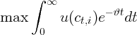(2)

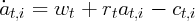
subject to the budget constraint

(3)

where the equality of the interest rates on capital and debt means that it does not matter how household net worth breaks down between assets and debt; all that matters for the budget constraint is total net worth.

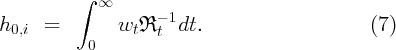
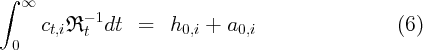
Integrating the household’s dynamic budget constraint and assuming a no-Ponzi-game transversality condition yields the intertemporal budget constraint, which says that the present discounted value of consumption must match the PDV of labor income plus the current stock of net wealth:

The formulas for these PDV’s are a bit awkward because they must take account of the fact that interest rates are varying over time. To make the formulas a bit simpler, define the interest factor

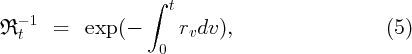
With this definition in hand we can write the IBC as

Each household solves the standard optimization problem taking the future paths of wages and interest rates as given. Thus the Hamiltonian¹ is

(8)

which implies that the first optimality condition is the usual u′(c_t,i) = λ_t,i. The second optimality condition is

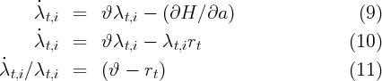
Note (for future use) that the RHS of this equation does not contain any components that are idiosyncratic: The consumption growth rate will be identical for all households. The same is true of the expression for human wealth, equation (7).

2 The Firm’s Problem

Now we assume that there are many perfectly competitive small firms indexed by j in this economy, each of which has a production function identical to the aggregate Cobb-Douglas production function. Perfect competition implies that individual firms take the interest rate _t and wage rate ŵ_t to be exogenous. Hence firms solve

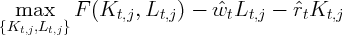(13)

where _t and ŵ_t are the rental rates for a unit of capital and a unit of labor for one period. Note that, dividing by L_t,j, this is equivalent to

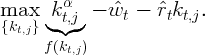(14)

The first order condition for this problem implies that

Under perfect competition firms must make zero profits in equilibrium, which means, by fact [EulersTheorem], that:

3 Equilibrium At a Point in Time

Thus far, we have solved the consumer’s and the firm’s problems from the standpoint of atomistic individuals. It is now time to consider the behavior of an aggregate economy composed of consumers and firms like these.

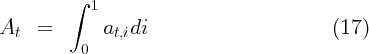
We assume that the population of households and firms is distributed along the unit interval and the population masses sum to one, as per Aggregation. Thus, aggregate assets at time t can be defined as the sum of the assets of all the individuals in the economy at time t,

Similarly, normalizing the population of firms to one yields

The first key assumption we will make is that all households and firms are identical. This assumption rules out the presence of any debt in equilibrium (if all households are identical, they cannot all be in debt - who would they owe the money to?). Indeed, in this case, the aggregate capital stock per capita will equal the aggregate level of net worth, k_t = a_t.²

Thus, households’ expectations about w_t and r_t determine their saving decisions, which in turn determine the aggregate path of k_t.

There is one important subtlety here, however. In writing the consumer’s budget constraint, we designated r_t as the net amount of income that would be generated by owning one more unit of net worth (e.g. capital). But if we have depreciation of the capital stock, the net return to capital will be equal to the gross return minus depreciation. The discussion of the firm’s optimization problem did not consider depreciation because the firms do not own any capital; instead, they make a payment _t to the households for the privilege of using the households’ capital. Thus the net increment to a household’s wealth if the household holds one more unit of capital will be

There is no depreciation of labor, so the labor market equilibrium will be

4 The Perfect Foresight Equilibrium

We assume that every household knows the aggregate production function, and understands the behavior of all the other households and firms in the economy. Understanding all of this, suppose that households have some set of beliefs about the future path of the aggregate capital stock per capita {k_t}_t=0^∞. This belief about k_t will imply beliefs about wages and interest rates as well {w_t,r_t}_t=0^∞.

The final assumption is that the equilibrium that comes about in this economy is the “perfect foresight equilibrium.” That is, consumers have the sets of beliefs such that, if they have those beliefs and act upon them, the actual outcome turns out to match the beliefs.

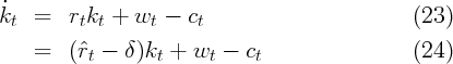
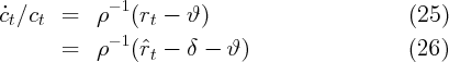
Note now that using the fact that a_t = k_t in the perfect foresight equilibrium we can rewrite the household’s budget constraint as

And we reproduce from (12)

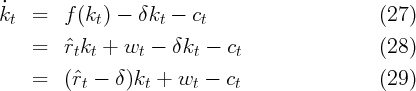
But compare these to the equations derived for the social planner’s problem (with population growth and productivity growth zero) in a previous handout:

Since the equilibrium value of _t = f′(k_t), (30) = (26). And (24) is identical to (29). Thus, aggregate behavior of this economy is identical to the behavior of the social planner’s economy!

This is a very powerful result, because it means that if we are careful about the exact assumptions we make we can often solve a social planner’s problem and then assume that the solution also represents the results that would obtain in a decentralized economy. The social planner’s solution and the decentralized solution are the same because they are maximizing the same utility function with respect to the same factor prices (r_t and w_t).

When will the decentralized solution not match the social planner’s solution? One important case is when there are externalities in the behavior of individual households; another possible case is where there is idiosyncratic risk but no aggregate risk; basically, whenever the household’s budget constraint or utility function differs in the right ways from the aggregate budget constraint or the social planner’s preferences, there can be a divergence between the two solutions.

References