The Benefits of Panel Data
in Consumer Expenditure Surveys
July 26, 2014


The Benefits of Panel Data
in Consumer Expenditure Surveys
July 26, 2014
_____________________________________________________________________________________
Abstract
This paper explains why the collection of panel (reinterview) data on a
comprehensive measure of household expenditures is of great value both for
measuring budget shares (the core mission of a Consumer Expenditure survey)
and for the most important research and public policy uses to which CE
data can be applied, including construction of spending-based measures
of poverty and inequality and estimating the effects of fiscal policy.
1Parker: MIT Sloan School of Management, JAParker@MIT.edu, 2Souleles: The Wharton School, University of Pennsylvania, 2300 Steinberg Hall - Dietrich Hall, Philadelphia, PA 19104-6367, e-mail: Souleles@Wharton.UPenn.edu, 3Carroll: ccarroll@jhu.edu, Department of Economics, 440 Mergenthaler Hall, Johns Hopkins University, Baltimore, MD 21218, and National Bureau of Economic Research.
Panel Data, Consumer Expenditure Survey, Survey Methods
E2, G1
| PDF: | http://www.econ2.jhu.edu/people/ccarroll/papers/ParkerSoulelesCarroll.pdf |
| Slides: | http://www.econ2.jhu.edu/people/ccarroll/papers/ParkerSoulelesCarroll-Slides.pdf |
| Web: | http://www.econ2.jhu.edu/people/ccarroll/papers/ParkerSoulelesCarroll/ |
| Archive: | http://www.econ2.jhu.edu/people/ccarroll/papers/ParkerSoulelesCarroll.zip |
|
“The Consumer Expenditure Survey (CE) program provides a continuous and comprehensive flow of data on the buying habits of American consumers. These data are used widely in economic research and analysis, and in support of revisions of the Consumer Price Index.” – Bureau of Labor Statistics (2009) |
Since the late 1970s, two features have distinguished the U.S. Consumer Expenditure (CE) Survey from any other American household survey: Its goal is to obtain comprehensive spending data (that is, not just in a few spending categories and not just over a brief time interval), and it has a panel structure (it reinterviews households, which enables measurements of how a given household’s spending changes over time).
These two features give the survey great value. This is why, in addition to satisfying the core mission of measuring the spending basket needed to construct the Consumer Price Index (CPI), the CE data are widely used by Federal agencies and policymakers examining the impact of policy changes, and by businesses and academic researchers studying consumers’ spending and saving behavior. These uses are rightly emphasized by the BLS, for example in the quote that begins this paper.
It could be argued that the non-CPI-related uses of the survey are becoming more important than its core use in constructing the CPI. After all, spending weights can be constructed from aggregate data without a household survey; many countries use such price indexes (often in the form of a ‘PCE deflator’) as their principal (or their only) measure of consumer inflation.2 And U.S. macroeconomic analysis has moved increasingly toward use of the PCE deflator instead of the CPI.3
But national-accounts-based spending weights do not provide any information about how expenditure patterns vary across households with different characteristics (e.g., elderly vs working-age, or employed vs unemployed, or any of myriad other subpopulations whose expenditure patterns might be important to measure). The BLS CE Survey homepage rightly emphasizes the point: “The CE is important because it is the only Federal survey to provide information on the complete range of consumers’ expenditures and incomes, as well as the characteristics of those consumers.”4 Furthermore, without expenditure data, it is impossible to measure the differing rates of inflation experienced by different kinds of households. These purposes provide a compelling case for continued collection of comprehensive spending data at the level of individual households.
The importance of maintaining the second of the CE’s two unique features – the panel aspect of the survey – is less obvious. Our purpose is to articulate and explore the reasons that the panel aspect of the data is extremely valuable. We argue that panel data contribute greatly to the central mission of the CE Survey, construction of the CPI (both the aggregate CPI and the relevant indexes for subgroups), as well as to its other missions, such as helping researchers and policymakers understand the spending and saving decisions of American households.
A panel survey is arguably more expensive and more difficult to conduct than a cross section survey would be,5 and any redesign of the CE Survey must consider costs as well as benefits. We do not have the expertise to estimate the costs of preserving the panel dimension of the survey, so our goal is simply to ensure that the significant benefits of true panel data on comprehensive spending be clearly recognized. Specifically, we focus on the following benefits, and their implications for CE redesign. Collection of panel data:
The rest of the paper considers each of these benefits in turn. Where we discuss the extant CE Survey we focus on the interview survey rather than its (also useful) diary complement. (For reasons that will become clear below, our view is that it is impossible for a diary survey to form the basis for a meaningful panel.)
This section discusses first how in a redesigned CE Survey repeated interviews can increase the accuracy of any given measure of spending in a period and thus may improve the quality of the comprehensive spending data that virtually every use of the CE survey relies upon, directly or indirectly. Second, the section shows that that because spending has volatile transitory components, understanding the evolution of inequality in true standards of living, or constructing price indexes for households with different patterns of expenditure, requires measurement of spending not just at a point in time but over a substantial interval of time. Such long-term spending information is best measured by repeated interviews (or a time-series of administrative data), in part because recall is imperfect.
Measurement error in the CE threatens all of its missions; and measurement error seems to be increasing. The fact that households are interviewed several times in the collection of panel data offers the potential to reduce the mismeasurement of expenditures for those households who participate in multiple interviews (nonsampling error), but it is possible that the added burden of a panel survey increases another kind of error: Sampling error that arises when the participants in a survey differ in systematic but unobservable ways from the population.6 We discuss these in turn.7
Research by BLS staff and others has demonstrated that the expenditure data that are recorded in the survey for a particular household may be inaccurate for a host of reasons, including problems of respondent misinterpretation of the survey questions, incorrect recall, or deliberate misrepresentation (for example, about purchases of alcohol or illegal drugs), or as a result of data processing errors due to mistakes in collecting, recording, or coding expenditure information. For all of these categories of error, the benefit of repeated measurement of expenditures is potentially large.
The first benefit of true panel data is that familiarity breeds accuracy. As households are re-interviewed, respondents become familiar with the process and so the quality of the responses is likely to rise. Having gone through at least one expenditure interview, the household can better keep information on hand to improve the accuracy and efficiency/speed of responses. Households may also mentally note purchases during a subsequent recall period that might previously have been forgotten. (The paper by Hurd and Rohwedder (2013) in this volume provides evidence supportive of these hypotheses; in the survey literature, these kinds of effects are called “panel conditioning.” See Shields and To (2005) for a discussion of some of the less favorable effects of such conditioning.)
It is possible that some of the gains from repeat interviews may be captured by an initial contact interview, as the current CE structure provides. In a household’s contact interview, the CE Survey procedures are explained to household members and information is collected so that the household can be assigned a population weight. The preparation includes suggestions on record keeping, such as keeping receipts and bills (e.g. utility bills), so that they can be consulted in the subsequent interviews. While surely helpful, such a preview of the survey procedures is unlikely to foster the degree of understanding that is gained by actually participating in the survey.
A second benefit of repeated interviews is that the survey-taker has the ability look for and double-check reporting errors or omissions and so can correct potential mismeasurement.8 The current computer program that Census Bureau surveyors use during interviews in the field is programmed with various procedures to double-check suspicious entries. The introduction of computer-assisted personal interviews in 2003 may have improved the quality of the CE data.9
With re-interview panel data, this benefit can be maintained by the new, improved version of the CE. A respondent who previously reported an expenditure on any category of regular spending, such as on mobile telephone service, cable television, mortgage payments, and so forth can be prompted for these categories because the software can add additional prompts based on the reports from the previous interview. Not only can this assist in omitted categories, but it can be used to improve amounts. A household who is guessing about past spending on cell phones, for example, could be prompted with their previous report, or prompted conditional on their previous report having been based on consulting a specific bill.
Repeat interviewing also allows the correction of past responses based on more accurate information in a subsequent interview. For example, a respondent who had a water bill to consult when responding in one interview could be asked whether, based on the history on their bill, their previous response was accurate. Or, a respondent who realizes that he is making a wild guess about spending in a particular category in a given interview might pay more attention to spending in that category as subsequent bills arrive, thus leading to a better estimate of spending in subsequent interviews.
Finally, evidence from the survey research literature suggests that memorable events tend to be subject to the “telescoping” problem: They may be remembered as being nearer in time than they actually are (Neter and Waksberg (1964)). Thus a purely cross-sectional CE might overstate spending on automobiles (for example) if respondents tended to remember automobile purchases well but tended to think that they were more recent than they actually were. Here, the benefit of repeated interviews is the ability to check responses against reports from the previous interview to correctly measure the spending during the actual period covered by the interview. For example, the surveyor could remind the household that in their prior interview (say, three months ago) they reported a car purchase and check whether a claim that they had purchased a new vehicle in the last three months really constituted the second purchase of a new vehicle in such a short time.10
In sum, when households participate in repeated interviews the accuracy of their responses is likely to improve measurement quality, through respondent familiarity, through comparison of responses across interviews, and through checking for errors in temporal recall. These benefits are more likely to be reaped when the interviews are closer together in time.
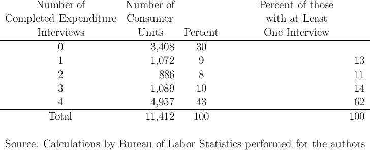
One widely acknowledged cost of repeated interviews is an increase in survey fatigue which leads some households to drop out of the survey without completing all interviews.11 Table 1 provides some statistics on the participation patterns for the 2008 survey (kindly provided to us by the BLS).12 The table indicates that while about 70 percent of households agreed to the first interview (the first row says 30 percent completed zero interviews), but only 43 percent completed all four interviews (last row). This compares with a corresponding full-interview-completion rate of 56.5 percent as recently as the late 1990s reported in Reyes-Morales (2003), who finds that households “who completed all four interviews are larger and older and are more likely to be homeowners and married couples than are [those] who responded only intermittently.”
These results suggest the potential for significant bias due to nonparticipation that is correlated with expenditure choices. If the households who complete all four interviews differ from those who complete only some, there can be little doubt that the households who refuse be interviewed at all (the 30 percent in the first row) differ systematically from those who complete at least one interview.13
It seems likely that the panel nature of the survey (specifically, the burden associated with reinterviews) increases the degree of sampling mismeasurement by introducing stronger selection effects than those that would exist for a single cross-section survey. To some extent this can be rectified in the construction of appropriate sample weights (for example, by reweighting the households who participate in multiple interviews so that the weighted sample’s characteristics match the characteristics of households who complete only a single interview). But to the extent that nonparticipation is both correlated with the expenditure of interest and not perfectly correlated with the observed household characteristics, the measurement of expenditures will be biased even after reweighting.
It is not clear, however, that the set of households who participate in the first interview are meaningfully different from those who would participate in a purely cross-section survey. Indeed, until the second interview is conducted, the CE survey is a cross-section survey.14 The size of the bias introduced as a result of reinterview-induced attrition might therefore be estimated by comparison of results obtained from a sample that includes only the first interview to results obtained from the complete CE dataset. If results are not markedly different, it may be that the reinterview-induced bias is not very large in its practical implications.
The case for measuring well-being using consumption rather than income goes back at least to Friedman (1957), whose famous “permanent income hypothesis” argued that income incorporates both permanent and transitory components, but that households choose their normal level of spending based principally on income’s permanent component. Friedman illustrated his argument by observing that households who are paid once a month do not concentrate all their spending on payday; rather, they choose a level of regular monthly expenditure (including mortgage payments, utility bills, etc) that on average matches the regular flow of income that they expect to receive. He then extended this point even to annual data; according to Friedman, households who experience transitory shocks to income in a given year will keep their expenditures close to the level of income expected in a “typical” year, smoothing through any temporary shocks to income.15
Nevertheless, most work on economic inequality has
focused on measuring disparities in household income, not
consumption16  17
This is likely because the CE data are not as well measured as the available income
data.18
17
This is likely because the CE data are not as well measured as the available income
data.18
What would be required for a redesigned CE to contribute significantly to the measurement of inequality? Two features stand out: comprehensive measures of spending, and measures that cover sufficiently long time periods without requiring recall over extended periods – that is, something like the panel structure of the current CE interview survey.
As Friedman noted, an important part of spending is on durable goods like cars, televisions, suits, and the like, which provide “consumption services” over a period far longer than the annual frequency of the budget survey. The theoretically correct measure of “consumption” would spread out the expenditures on such goods over the time span over which they provide value, rather than recording the entire expenditure as consumption on the date of purchase.
Friedman also emphasized the point that spending on nondurable goods and services may contain nonrepeating or transitory elements that do not reflect the household’s perception of its permanent income. For example, emergency vehicle repairs induced by an auto accident should not be confused with permanent elements of consumption.19
Friedman’s insightful original discussion of these points provides some enduring guidance about the appropriate goals of a redesigned CE survey. For example, it clarifies why spending data that cover a narrow slice of time (like a month or less) may provide a poor picture of both households’ true spending patterns across categories of goods and their long-term well-being. In only a short period, a household’s spending even on highly nondurable goods like food may be seriously distorted by economically meaningless variations like a long holiday or failure to visit the grocery store during one of the four weeks in the month.20
Over how long a period should spending be measured?
It seems plausible to propose that three months’ worth of spending data would provide a reasonable measure of a household’s usual spending on most nondurable goods including food. For example, using UK scanner data, Leicester (2013) shows that over a 4 week period about 8 percent of households recorded no spending on sugars or confectionary, but over a 12 week period only about 1 percent reported no spending in these categories. More broadly, he calculates the distribution across households of budget shares on various categories of commodities purchased at grocery stores when the data are aggregated at frequencies ranging from 2 weeks to a full year. For these highly non-durable goods, the distribution of budget shares for the three-month time interval are not sharply different from those for the yearly time interval, while the distribution of budget shares at the monthly frequency is markedly different. This evidence strongly supports the proposition that a month is not a long enough time interval to reliably measure a household’s usual spending behavior.
For more durable goods, Leicester (2013)’s data show that expenditure patterns over even a three month interval differ markedly from those over a full year. This is perhaps not surprising, since many kinds of spending – holiday travel, school expenses, clothing – vary systematically across households and are highly seasonal, or have a once-a-year character. (This is called the “infrequency of purchase” problem in the survey literature).
While these points suggest that longer interview timeframes might provide better measurement, such a conclusion might not be correct because longer periods might introduce other measurement problems. If respondents had perfect memories, an annual accounting could be accomplished in a single interview, but experience has shown that there are enormous measurement problems associated with long recall periods – forgotten expenditures, misremembered timing of purchases, and problems due to the burden of the length of interview required for such an long recall period.
With cross-sectional surveys there is always a trade-off in the recall period. Longer recall periods have greater recall problems (forgetting, telescoping, and so on) but shorter periods have more problems because of infrequency of purchase. A panel survey with repeated interviews dodges this tradeoff: Several interviews over which fluctuations in purchases can be averaged are likely to provide a much better measure of a household’s typical budget constraint and standard of living than can be obtained from a single interview.
Credible measurements of permanent expenditures are especially important for the CE’s mission of permitting the construction group-specific price indexes, which are a major advantage of a CE-based CPI over an inflation index constructed from aggregate spending weights.21 As an important example, an expenditure survey that accurately measures ‘permanent consumption’ can be used to measure price indexes for households at different levels of standards of living. Broda and Romalis (2009) for example show that high and low expenditure households have experienced substantially different changes in the prices of the baskets of the goods that they consume so that the inequality in the nominal expenditure levels of these different groups of households overstates the increase in inequality in real expenditure between groups.
The mandate to improve the usefulness of the CE for measuring poverty provides an important further reason for collecting panel data (as “poverty” defined by expenditure ought to be based on permanent expenditure patterns). When short time intervals are employed, infrequency of expenditure generates spurious dispersion that does not correspond to meaningful variation in standards of living.
A final related point is that the collection of panel data could prove to be important for the CE’s ability to meet future needs that are not currently anticipated. A plausible example of such a use might be the construction of a price index for people with “high medical expenses.” If only cross-section data were available, the price index would inevitably be biased (lumping together, say, people with temporarily high expenses because of an auto accident, with people with permanently high expenses because of a chronic condition). It would be impossible to construct a credible price index for such a group without panel data.
|
“The mission of the Consumer Expenditure Survey program (CE) is to collect, produce, and disseminate information that presents a statistical picture of consumer spending for the Consumer Price Index, government agencies, and private data users. The mission encompasses analyzing CE data to produce socio-economic studies of consumer spending …” – Horrigan (2011). |
An alternative to true panel data is synthetic panel data. Such data can be useful for some purposes, but the section following this one lays out some the limitations of synthetic panel data.
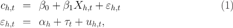
Consider the following general framework for studying the causal impact of some
observed variable  for household
  and time
  on the expenditure of that
household
on the expenditure of that
household  .
.
In this statistical model, we assume additivity of the unobserved
determinants of spending, denoted  , and assume that the causal
effect, given by
, and assume that the causal
effect, given by  , is linear and homogeneous across households and
time. Neither assumption is central to the issues we discuss but both
make our points easier to elucidate. Notably, we assume that there is a
permanent household-specific component of
, is linear and homogeneous across households and
time. Neither assumption is central to the issues we discuss but both
make our points easier to elucidate. Notably, we assume that there is a
permanent household-specific component of  , denoted
  , and
potentially a time-specific component common across households, denoted
, and
potentially a time-specific component common across households, denoted
 .23
.23
The analysis of this equation could proceed, given certain strong assumptions, using cross-sectional data alone.
As an alternative, one could, given repeated observations on spending of the same households over time, first-difference equation (1) and analyze the change in spending over time:
Notice that the individual effect ( ) drops out. The advantages of this equation
then stem, first, from the ability to estimate the causal effect
) drops out. The advantages of this equation
then stem, first, from the ability to estimate the causal effect  consistently
when there is possible correlation between
consistently
when there is possible correlation between  and
and  in the cross-section,
and, second, from increased power in the first-difference estimation because
the variation in
in the cross-section,
and, second, from increased power in the first-difference estimation because
the variation in  generally weakens estimation of the relationship of
interest.
generally weakens estimation of the relationship of
interest.
An important caveat is that (2) will be biased if  is measured with
error. We discuss the implications of such measurement error below, which
has varying plausibility for different
is measured with
error. We discuss the implications of such measurement error below, which
has varying plausibility for different  variables. But for clarity of
exposition we begin with the assumption that
variables. But for clarity of
exposition we begin with the assumption that  has no measurement
error.
has no measurement
error.
In many applications, it is unreasonable to expect that persistent, unmodelled
differences in household expenditure levels are uncorrelated with the variation in
 across households. If
 ![E [α |X ] ⁄= 0](ParkerSoulelesCarroll27x.png) , then cross-sectional estimation of
, then cross-sectional estimation of  is inconsistent. As an example, consider a study of how tax rates are related to
expenditures. In a cross-section of households, wealthier households will tend to
have higher levels of expenditure and higher tax rates, so the relationship
uncovered by estimation of equation (1) would be that households with higher
tax rates would tend to have higher expenditures,
is inconsistent. As an example, consider a study of how tax rates are related to
expenditures. In a cross-section of households, wealthier households will tend to
have higher levels of expenditure and higher tax rates, so the relationship
uncovered by estimation of equation (1) would be that households with higher
tax rates would tend to have higher expenditures,  . Obviously, it would
be a mistake to conclude from this that raising tax rates would raise household
expenditures.
. Obviously, it would
be a mistake to conclude from this that raising tax rates would raise household
expenditures.
One solution would be to try to include measures of permanent income and wealth on the right had side of the equation (1) to ‘control for’ differences in household-specific spending levels not driven by tax rates. While this might seem straightforward, in order to eliminate the bias, the measure of permanent income used must capture all the variation in permanent income. Thus, as already discussed, one needs not just to capture variation in current income and wealth, but enough variables to capture completely any differences in household-specific variation in anticipated future income that might be correlated with tax rates. This is surely impossible (although absorbing most of the variation would eliminate most of the bias).
A common, and better, solution is to focus on the sort of variation that
identifies what is probably the effect of interest: how a change in taxes changes
the expenditures of households on average. To do this, one can measure the
average relationship between the change in expenditures and the change in
tax rates over time, as in equation (2). This relationship removes the
household-level effect,  , which is the problematic term causing the
inconsistency in equation (1). (Of course, one also might expect the
true effect
, which is the problematic term causing the
inconsistency in equation (1). (Of course, one also might expect the
true effect  to differ with household characteristics. But allowing for
different effects in different subpopulations is straightforward using equation
(2).)
to differ with household characteristics. But allowing for
different effects in different subpopulations is straightforward using equation
(2).)
Formally, when ![E [α |X ] ⁄= 0](ParkerSoulelesCarroll32x.png) estimates of
estimates of  using equation (1) are biased.
One can still estimate
using equation (1) are biased.
One can still estimate  consistently if in addition to
  one includes a vector
of
one includes a vector
of  of persistent household-level characteristics that completely capture all
variation in
of persistent household-level characteristics that completely capture all
variation in  and is orthogonal to
  ,
, ![E [ε|X, Z ] = 0](ParkerSoulelesCarroll39x.png) . But even this
approach is still likely to be less efficient than panel data estimation (as we show
below).
. But even this
approach is still likely to be less efficient than panel data estimation (as we show
below).
Our example may seem special because it focuses on the change in spending over time, rather than the level. But most questions of either academic or policy interest are of the form: “How does some change in the environment change spending?” A topical example important to the macroeconomic outlook as this paper is being written is the effect of changes in housing prices on spending (the ‘housing wealth effect’). Cross section data would undoubtedly show that people with greater housing wealth have greater consumption expenditures, controlling for any and all other observable characteristics, but a substantial part of this relationship would surely reflect the fact that people with higher unobserved permanent income have both higher spending and higher wealth. The causal effect of house price shocks on spending would remain unknowable. Similarly, the effects on household spending of policy interventions designed to induce mortgage refinancing cannot be plausibly estimated with cross section data, for the same reasons. These examples are the norm, not the exception. Indeed, few variables spring to mind that would be directly related to household consumption expenditures but would not also be systematically related to the unobservable determinants of consumption like permanent income.
But a solution comes from the permanent income theory of consumption. The theory implies that for an optimizing consumer the path of spending will satisfy an equation like:
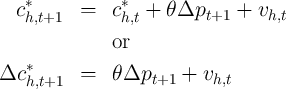
 might represent the change in the real price of
goods between two periods, that is, the real interest rate between these
periods. This is the famous ‘random walk’ proposition of Hall (1978). In
this analysis, the key question of interest is the coefficient
might represent the change in the real price of
goods between two periods, that is, the real interest rate between these
periods. This is the famous ‘random walk’ proposition of Hall (1978). In
this analysis, the key question of interest is the coefficient  which
reveals the effect of the interest rate (say) on consumption growth. More
sophisticated versions of the theory allow roles for uncertainty, liquidity
constraints, and other variables, but still tend to assign a central role to the
change in consumption as a measure of the change in circumstances.
According to these theories, the change in spending is the most fundamental
appropriate object of analysis. This key point explains the exalted role that
panel data (even when it comes in highly problematic forms like “usual”
household food expenditures) has played in the academic and policy
literatures.
which
reveals the effect of the interest rate (say) on consumption growth. More
sophisticated versions of the theory allow roles for uncertainty, liquidity
constraints, and other variables, but still tend to assign a central role to the
change in consumption as a measure of the change in circumstances.
According to these theories, the change in spending is the most fundamental
appropriate object of analysis. This key point explains the exalted role that
panel data (even when it comes in highly problematic forms like “usual”
household food expenditures) has played in the academic and policy
literatures.
The previous section shows the benefits of panel data when ![E [ε |X ] ⁄= 0](ParkerSoulelesCarroll43x.png) . A
next question is whether panel data is important even when
. A
next question is whether panel data is important even when ![E [ε|X ] = 0](ParkerSoulelesCarroll44x.png) . For
the reasons sketched above, this is typically an implausible assumption, but we
maintain it throughout this subsection to illustrate that there can be important
improvements in the precision of estimation from using true panel data rather
than cross-sectional data in this case. These advantages arise from the ability to
eliminate the variation stemming from
. For
the reasons sketched above, this is typically an implausible assumption, but we
maintain it throughout this subsection to illustrate that there can be important
improvements in the precision of estimation from using true panel data rather
than cross-sectional data in this case. These advantages arise from the ability to
eliminate the variation stemming from  across households. (For a
comprehensively useful treatment of the issues discussed below and many related
ones, see Deaton (2000b); for a more general-purpose treatment, see Johnston
and DiNardo (2000); and for a clear discussion of panel identification issues,
see Moffitt (1993)).24
across households. (For a
comprehensively useful treatment of the issues discussed below and many related
ones, see Deaton (2000b); for a more general-purpose treatment, see Johnston
and DiNardo (2000); and for a clear discussion of panel identification issues,
see Moffitt (1993)).24
To make this point as concretely as possible, consider cross-sectional (CS)
estimation of the effect of interest denoted  with sample size
  , and
first-difference (FD) estimation on true panel data denoted
, and
first-difference (FD) estimation on true panel data denoted  , also
with sample size
, also
with sample size  (for example, two cross-sections on the same
  households).25
If ![E [ε |X ] = 0](ParkerSoulelesCarroll51x.png) (and our other assumptions hold), both estimators are
unbiased. But the asymptotic approximation to the statistical uncertainty is
smaller for the estimator of
(and our other assumptions hold), both estimators are
unbiased. But the asymptotic approximation to the statistical uncertainty is
smaller for the estimator of  using equation (2) and true panel data than
for the estimator of
using equation (2) and true panel data than
for the estimator of  using equation (1) and cross-sectional data if
var
using equation (1) and cross-sectional data if
var var
var . Assuming (for the moment) that
  and
and  are
independent and identically distributed across
are
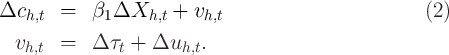
independent and identically distributed across  in each sample, the asymptotic
approximations to these variances are:
in each sample, the asymptotic
approximations to these variances are:
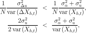
To further interpret these equations, assume temporarily that  and
and  are
independent and identically distributed over time so that
are
independent and identically distributed over time so that  and
and
 . Under these (admittedly extreme) assumptions, the
panel-data first-difference estimator is more efficient than the cross-sectional
data levels estimator if
. Under these (admittedly extreme) assumptions, the
panel-data first-difference estimator is more efficient than the cross-sectional
data levels estimator if
 |
While  and
and  are highly unlikely to be independent over time, the
intuition for this result is broadly useful and intuitive: A second observation on a
given household provides more information than a first observation on a different
household because, as long as there are persistent household effects, the first
observation tells you something (and may tell you a lot) about what to
expect for the second (and vice versa). Intuitively, with less statistical
uncertainty surrounding the possible determinants of the expenditures
that one is trying to explain with
are highly unlikely to be independent over time, the
intuition for this result is broadly useful and intuitive: A second observation on a
given household provides more information than a first observation on a different
household because, as long as there are persistent household effects, the first
observation tells you something (and may tell you a lot) about what to
expect for the second (and vice versa). Intuitively, with less statistical
uncertainty surrounding the possible determinants of the expenditures
that one is trying to explain with  , the role of
  is easier to
measure.
is easier to
measure.
This conceptual point gains empirical clout from the fact, widely known among
microeconomists, that observable  variables have embarrassingly little
explanatory power for expenditures, income, wealth, or other similar outcomes in
cross-section regressions. It is rare to encounter a dataset in which a dependent
variable relevant to our discussion can be explained with an
variables have embarrassingly little
explanatory power for expenditures, income, wealth, or other similar outcomes in
cross-section regressions. It is rare to encounter a dataset in which a dependent
variable relevant to our discussion can be explained with an  is greater than
0.5. The traditional interpretation of this fact is that unmeasured variables are
hugely important in practice; and it is not implausible to guess that most such
variables are highly persistent.
is greater than
0.5. The traditional interpretation of this fact is that unmeasured variables are
hugely important in practice; and it is not implausible to guess that most such
variables are highly persistent.
Exploring our setup further, it is also useful to think about the polar
alternative to an iid  ; if
; if  is perfectly persistent,
  and
and  collapses to zero. This implausible result highlights (among other things) the
extreme nature of our assumptions that
collapses to zero. This implausible result highlights (among other things) the
extreme nature of our assumptions that  is measured without error (and,
implicitly, that
is measured without error (and,
implicitly, that  has nonzero variance). But it also makes very clear the
point that the more important are persistent unmodeled differences in
spending, the more useful is panel data for obtaining power in any given
inference.
has nonzero variance). But it also makes very clear the
point that the more important are persistent unmodeled differences in
spending, the more useful is panel data for obtaining power in any given
inference.
Another lesson of (3) is about the great importance (in the panel context) of
minimizing or eliminating measurement error in  (though perfectly
persistent measurement error in the level of
(though perfectly
persistent measurement error in the level of  is not a problem). It is easy to
see that such measurement error will bias the estimates of
is not a problem). It is easy to
see that such measurement error will bias the estimates of  (toward zero, in
the univariate case); (3) makes plain that such error will also bias down the
measured variance of the panel estimator. The upshot is that, while good
measurement is important in a cross-section context, it may be even
more important in a panel context. This point could be important in
guiding survey designers among the choices they must make; if survey
resource constraints force a choice, say, between collecting several variables
that have high transitory measurement error and one that has little
or no measurement error, the logic of panel estimation would tend to
suggest a very high value to collecting the variable with low measurement
error.
(toward zero, in
the univariate case); (3) makes plain that such error will also bias down the
measured variance of the panel estimator. The upshot is that, while good
measurement is important in a cross-section context, it may be even
more important in a panel context. This point could be important in
guiding survey designers among the choices they must make; if survey
resource constraints force a choice, say, between collecting several variables
that have high transitory measurement error and one that has little
or no measurement error, the logic of panel estimation would tend to
suggest a very high value to collecting the variable with low measurement
error.
A few caveats now deserve mention.
First, less persistence in  (a greater value of the household-specific error
term
(a greater value of the household-specific error
term  ) weakens the panel data estimator. For questions in which
expenditures are the object to be explained, classical measurement error will not
bias estimates of
) weakens the panel data estimator. For questions in which
expenditures are the object to be explained, classical measurement error will not
bias estimates of  , but will reduce their precision. But in some contexts
expenditures are an independent rather than a dependent variable; there,
measurement error could lead to bias as well.
, but will reduce their precision. But in some contexts
expenditures are an independent rather than a dependent variable; there,
measurement error could lead to bias as well.
Second, and in many contexts more problematic, the more persistent  is
over time, the less variation there is in
is
over time, the less variation there is in  (holding its cross-sectional variance
fixed). For many potential
(holding its cross-sectional variance
fixed). For many potential  variables (e.g., demographics) first differencing
removes all information since the household’s demographic characteristics usually
do not change over time. Since the first-difference estimator relies on this
variation to identify the effect of interest, it is weaker when there is less variation
in this dimension.
variables (e.g., demographics) first differencing
removes all information since the household’s demographic characteristics usually
do not change over time. Since the first-difference estimator relies on this
variation to identify the effect of interest, it is weaker when there is less variation
in this dimension.
A generalized least squares estimator like the random effects estimator would balance these benefits and weight the variation in the different dimensions to produce a still more efficient estimator. But the main point remains, that repeated observations on the same households – because each observation provides more information about the other than either would about a third, random household – can enhance the power of estimation in the presence of unmodelled persistent differences in household spending levels. And this logic carries over to a large class of nonlinear and more complex models than considered here.
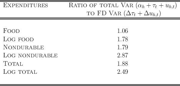
How important are these issues in practice in the current CE survey? For
illustrative purposes, we calculate the variances that affect the power of panel
vs. cross-sectional estimation using CE Interview Survey data from the family
files in 2007 and 2008. Since no single application is critical, we simply assume
that  and consider no
  in our calculations. Table 2 shows the ratio of
the variances in equation (3) based on estimation of equations (1) and (2) under
the assumption that
in our calculations. Table 2 shows the ratio of
the variances in equation (3) based on estimation of equations (1) and (2) under
the assumption that  and
and  , and
, and  are independent and identically
distributed. For the cross-sectional regression, we ignore the panel structure in
estimation and inference, treating the data as if there were no repeat interviews
of the same household.
are independent and identically
distributed. For the cross-sectional regression, we ignore the panel structure in
estimation and inference, treating the data as if there were no repeat interviews
of the same household.
Table 2 shows that estimates from panel data (would) have roughly half the
variance of the corresponding analysis pretending that the data was purely
cross-sectional in nature. While the actual improvement will depend on the
specific analysis, these results suggest that standard errors on coefficients of
interest could be about  smaller when a first-difference estimator is used
and likely smaller still if a random effects estimater were employed (which
would be consistent if the cross-sectional analysis were also consistent).
Furthermore, in many applications the assumptions necessary for consistent
estimation in cross-sectional data are not met, so that power is irrelevant
and the only way to make inference at all is to have access to panel
data.
smaller when a first-difference estimator is used
and likely smaller still if a random effects estimater were employed (which
would be consistent if the cross-sectional analysis were also consistent).
Furthermore, in many applications the assumptions necessary for consistent
estimation in cross-sectional data are not met, so that power is irrelevant
and the only way to make inference at all is to have access to panel
data.
A final important point concerns the limits to the advantages of panel data for
power. As with the case where ![E [α |X ] ⁄= 0](ParkerSoulelesCarroll94x.png) so that cross-sectional estimation is
inconsistent, it is possible to improve power in the cross-section by modelling
so that cross-sectional estimation is
inconsistent, it is possible to improve power in the cross-section by modelling  .
As in the previous case, any included
.
As in the previous case, any included  must be orthogonal to
  to preserve
consistency. But, what we did not note in the previous section, these additions
can be costly in terms of power. As one introduces more variables in the vector
of
to preserve
consistency. But, what we did not note in the previous section, these additions
can be costly in terms of power. As one introduces more variables in the vector
of  , one introduces more parameters to estimate which lowers the
precision of the estimator, leading to a (at least partially) offsetting increase
in the variance of
, one introduces more parameters to estimate which lowers the
precision of the estimator, leading to a (at least partially) offsetting increase
in the variance of  . Further, to the extent that these additional
variables are correlated with
. Further, to the extent that these additional
variables are correlated with  , their addition further increases in
the variance of
, their addition further increases in
the variance of  . The additional variables do this by leaving less
independent variation in
. The additional variables do this by leaving less
independent variation in  from which to identify the effect of
  on
spending. Finally, it is possible that the additional covariates also reduce
the variance of household-specific non-persistent unmodeled variation;
that is, they may reduce the variance of
on
spending. Finally, it is possible that the additional covariates also reduce
the variance of household-specific non-persistent unmodeled variation;
that is, they may reduce the variance of  . To the extent that these
covariates reduce this variation, they can actually raise the precision of
. To the extent that these
covariates reduce this variation, they can actually raise the precision of
 and reduce its variance. In this case, if these covariates vary over
time, they can also increase the power and reduce the variance of the
panel data estimator. In sum, while in theory it is possible to model
permanent household-level determinants of spending levels and approach the
precision of estimation that exploits the panel dimension of panel data,
it is rarely the case in practice that there are sufficiently few actually
exogenous determinants of persistent differences to make cross-sectional data
on spending as powerful as the comparable dataset with a true panel
dimension.
and reduce its variance. In this case, if these covariates vary over
time, they can also increase the power and reduce the variance of the
panel data estimator. In sum, while in theory it is possible to model
permanent household-level determinants of spending levels and approach the
precision of estimation that exploits the panel dimension of panel data,
it is rarely the case in practice that there are sufficiently few actually
exogenous determinants of persistent differences to make cross-sectional data
on spending as powerful as the comparable dataset with a true panel
dimension.
In this subsection we present an example that illustrates the importance of the benefits of panel data just discussed. We consider how the availability of panel data affects the ability to study the effect of the receipt of a stimulus tax rebate on spending, following Parker, Souleles, Johnson, and McClelland (2011).
Parker, Souleles, Johnson, and McClelland (2011) use the CE Survey to measure the effect of the receipt of a 2008 Economic Stimulus Payment (ESP) on spending during the three months of receipt. The BLS working with the authors added a supplement to the standard survey to cover this additional source of household income in sufficient detail to allow the research. The BLS was able to accomplish this extremely rapidly, as the time between the law that enacted the stimulus payment program and the first payments was only a few months.26 The ESPs were distributed by the Federal government from the end of April to the beginning of July 2008. The amount of payment any household received was based on year-2007 taxable income. The timing of the receipt was determined largely by the last two digits of the tax filer’s social security number and the means of delivery – electronic transfer of funds or mailed paper check.27
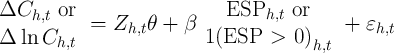
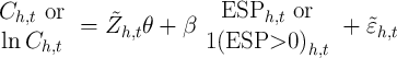
Parker, Souleles, Johnson, and McClelland (2011) estimate the following equation
 | (4) |
where the dependent variable is three-month to three-month change in spending
or log spending, the control variables,  , are age of household head, change
in the number of children, and change in the number of adults, and the key
independent variable is either the stimulus payment amount received in
that period or an indicator for whether any payment is received in that
period.
, are age of household head, change
in the number of children, and change in the number of adults, and the key
independent variable is either the stimulus payment amount received in
that period or an indicator for whether any payment is received in that
period.
To illustrate the importance of panel data, we consider instead the estimated effect of receipt of a stimulus payment on spending from a regression that is analogous to equation (4) but in levels instead of first-differences.
 | (5) |
where the vector of control variables,  , are age, age-squared, the number of
children and the number of adults.
, are age, age-squared, the number of
children and the number of adults.
There are several reasons why estimation in first-differences is more likely to lead to consistent estimation of the causal effect of stimulus payments. First, whether a household receives a rebate at all is a function of previous year’s income, which in turn is correlated with standard of living. Thus, in the entire sample, there is a correlation between the level of income and payment receipt that does not reflect the causal effect of the receipt of a payment on spending, but instead partly measures the effect of permanent income on both spending and eligibility for a payment. While there is the possibility that this type of problem might arise in first differences, it is less likely. Nevertheless, it is possible that households ineligible for stimulus payments in a given period have different changes in spending (or log spending) than the typical recipient. For this reason, Parker, Souleles, Johnson, and McClelland (2011) focus most of their analysis on the subsample of households that report receiving a payment and we follow this choice and focus only on households that recieve stimulus payments at some point in time.
The second reason to estimate in first differences applies to this subsample. The amount of the stimulus payment is determined by household characteristics, such as income (eligibility for reciept of the payment required a minimum income and was phased out at high incomes) and the number of children eligible for the child tax credit. First-differencing implies that any correlation between the level of spending and stimulus payment caused by permanent income or usual standard of living is removed from the variation that identifies the causal effect of the payment on spending. There remains a smaller concern that this type of correlation might cause bias even in first differences due to a correlation between spending changes and other factors correlated with household characteristics. To circumvent this concern, the original analysis also considers the effect of stimulus payment receipt; we do so here also.
Table 3 shows the results of estimation of equation (4) in the top panel and equation (5) in the bottom panel. The coefficients in the first and third pairs of columns are interpreted as the proportion of the stimulus payment spent during the three month period in which it is received. The middle two colums show the percent increase in spending upon receipt. The final row shows the percent by which the cross-sectional estimates differ from the panel estiamtes. These differences are large, in some cases more than 100 percent. They are large and negative for the analysis with a log dependent variable despite the fact that these results use only variation in the timing of receipt (the middle pair of columns of results). And the bias is larger for nondurable than for durable goods.
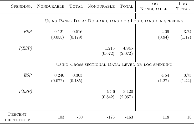
Source of data: Parker, Souleles, Johnson, and McClelland (2011) Regressions on the bottom use the same sample in cross-sectional form, so the dependent variable is level or log consumption and the controls add age squared and are number of kids and num of adults instead of changes. All regressions include a complete set of time dummies.
Many interesting issues in the analysis of spending data involve not just the contemporaneous effect on spending of a contemporaneous change in environment but the dynamics of this effect over time.
Consider for example, the research on aggregate consumption expenditures
that shows that they are ‘too smooth’ to be explained by standard versions of
the canonical permanent-income model. A common response has been to
incorporate ‘habit formation’ into the utility function in aggregate models, so
that changes in circumstances lead to persistent dynamic changes in spending
(because habits slow the adjustment of consumption to changed circumstances).
In one of the main models of habits for example, the strength of the habit
formation motivation can be estimated as the coefficient  in a regression of
the form
in a regression of
the form

 . Across thirteen countries, Carroll, Sommer, and Slacalek (2011)
find an average value of
. Across thirteen countries, Carroll, Sommer, and Slacalek (2011)
find an average value of  , with no country having a point estimate
below 0.5.
, with no country having a point estimate
below 0.5.
Many other kinds of models (for example, models with sticky expectations or rational inattention) also predict important and extended dynamics of spending. In the economic stimulus example of the previous section, a central question is whether the stimulus-related spending was rapidly reversed so as to provide little net increase in spending over longer periods like six months or nine months. The current panel structure of the CE (with 3 first-differences in expenditures) allowed this to be investigated.
Another (related) set of interesting questions concerns the degree of “mobility” in expenditure patterns. A large literature has measured the degree of income mobility as a proxy for socioeconomic fluidity; but if consumption determines utility, mobility (or the lack of mobility) in spending should be even more interesting than income mobility. Measuring spending mobility in this sense, of course, requires comprehensive panel data on spending over an extended period, at least a few years, which may not be feasible for a CE-type survey. In principle, such questions might be addressed, however, by survey data from sources like the Panel Study on Income Dynamics using its new questions that attempt to measure broad aggregates of household spending. An improved CE survey with a shorter panel element, however, could play a vital role in calibrating the degree of measurement error versus true mobility that would emerge from a PSID-type study.
Because extended dynamics are central to the questions posed by these
models, panel data are indispensable to being able to answer them. Cross-section
data offer virtually no ability to estimate parameters like  . Of course,
estimation of such a parameter can be problematic even in panel data, because
any measurement error or transitory variation in lagged consumption growth
should bias the
. Of course,
estimation of such a parameter can be problematic even in panel data, because
any measurement error or transitory variation in lagged consumption growth
should bias the  coefficient toward zero. But in principle, careful econometric
work (and assumptions about the size and nature of the transitory ‘noise’) could
yield estimates of
coefficient toward zero. But in principle, careful econometric
work (and assumptions about the size and nature of the transitory ‘noise’) could
yield estimates of  that should be comparable to those from macro data. (See
Dynan (2000) for just such an effort.) Without high-quality panel data on
household-level spending, it will likely be impossible to distinguish between
the competing explanations (habits, sticky expectations, etc) for the
macroeconomic stickiness of consumption growth. This matters, because
alternative interpretations have quite different consequences for vitally important
questions like the appropriate monetary and fiscal policies during an economic
slump.
that should be comparable to those from macro data. (See
Dynan (2000) for just such an effort.) Without high-quality panel data on
household-level spending, it will likely be impossible to distinguish between
the competing explanations (habits, sticky expectations, etc) for the
macroeconomic stickiness of consumption growth. This matters, because
alternative interpretations have quite different consequences for vitally important
questions like the appropriate monetary and fiscal policies during an economic
slump.
By grouping or averaging repeated cross-sections on time-invariant household characteristics, a researcher can track group averages over time and conduct panel analysis for cohorts as unit of observation, as for example
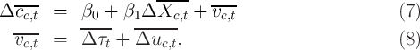
The CE data have been fruitfully used for such analyses, for example by Attanasio and Weber (1995), Gourinchas and Parker (2002) and Attanasio and Davis (1996). Attanasio and Weber (1995) studies how consumption growth responds to changes in interest rates. In this case, averaging loses the researcher very little within-cohort variation in the key explanatory variables because most of the power of the analysis comes from changes over time. Further, as exemplified by Gourinchas and Parker (2002), in practice, estimation from moments requires that the moments that are available for every household be collapsed to average moments across households in the finite sample (otherwise there are far too many moments for the data size for any hope for GMM asymptotics to apply). When moments like this are employed, even analyses that use true panel data (such as Attanasio and Vissing-Jorgensen (2003) for example) take cross-sectional averages before estimating. In the case of Attanasio and Davis (1996), to match data across unrelated datasets requires the construction of synthetic cohorts in any case, so that true panel data is of less use. Another example is Aaronson, Agarwal, and French (2011) who study the effect of a change in the minimum wage on spending by comparing changes in households’ spending around dates when state-specific minimum wages were changed. Since the change in the minimum wage is statewide, no information is lost by collapsing the data across states.
Perhaps the greatest shortcoming of synthetic panel analysis is the
enormous loss of variation in the independent variable that could have
been used to identify the effect of interest. The significance of this loss
depends on the relative variances of the independent variables and the
residual in the true panel data and in the synthetic equivalent, that is on
var and
and  vs.
vs.  and
and  . In the
extreme case, if there is no variation in
. In the
extreme case, if there is no variation in  that is correlated with
cohort characteristics, then one loses identification completely in synthetic
cohorts.
that is correlated with
cohort characteristics, then one loses identification completely in synthetic
cohorts.
Any randomized experiment, like the timing of economic stimulus payments
among recipients, has no (asymptotic) variation at the synthetic cohort
level. That is, the best possible source of variation – variation that is
independent of households’ characteristics – is impossible to exploit in
a panel dimension using synthetic cohort analysis. In general, in any
situation where  with the size of the cohorts, there is no
exploitable variation in synthetic panel data (but there would be in true panel
data.)
with the size of the cohorts, there is no
exploitable variation in synthetic panel data (but there would be in true panel
data.)
A second relative shortcoming of synthetic panel data is that it can be impossible (or sometimes difficult, requiring many other assumptions) to identify the change in spending for a time-varying population of interest. For example, researchers have been interested in measuring the consumption of stockholders or might be interested in measuring the effect of house-price changes on spending. But households’ stockholding status can switch over time (if they buy or sell their portfolio), and even more obviously homeownership status can change. This significantly impedes analysis. Attanasio and Vissing-Jorgensen (2003) thus use the true panel nature of the CE Survey and Attanasio, Banks, and Tanner (2002) need additional information and must make additional assumptions to show that their estimates will be unbiased because they use only cross-sectional data.
The CE survey can be used to address many economically crucial questions that no other U.S. survey can be used to address. This reflects two important features that are therefore valuable to maintain in any redesign of the CE survey. The first of the CE’s unique characteristics is its collection of spending data that is comprehensive in both the scope of expenditures and the span of time covered. This need is compelling but obvious, so our paper focuses on articulating the value provided by the second of the unique features of the CE survey: its provision of household-level true panel data on spending.
A re-interviewing process that yields true panel data on spending is critical to the core missions of the CE survey, such as the construction of group-specific price indices or improving the measurement of poverty. Panel data is even more important for the the many research purposes to which the survey has been put, such as estimating the marginal propensity to consume out of economic stimulus payments.
The BLS faces formidable challenges in redesigning the survey in a way that preserves its current unique qualities and addresses the growing problems of measurement error. But any redesign would be a large step backwards if it did not preserve both the comprehensiveness and the panel features of the current survey.
AARONSON, DANIEL, SUMIT AGARWAL, AND ERIC FRENCH (2011): “The Spending and Debt Response to Minimum Wage Hikes,” Federal Reserve Board of Chicago Working Paper, 2007-23, 14.
AGUIAR, MARK A., AND MARK BILS (2011): “Has Consumption Inequality Mirrored Income Inequality?,” NBER Working Paper 16807, National Bureau of Economic Research, Inc.
ATTANASIO, ORAZIO, JAMES BANKS, AND SARAH TANNER (2002): “Asset Holding and Consumption Volatility,” Journal of Political Economy, 110(4), 771–92.
ATTANASIO, ORAZIO, ERICH BATTISTIN, AND HIDEHIKO ICHIMURA (2004): “What Really Happened to Consumption Inequality in the US?,” NBER Working Papers.
ATTANASIO, ORAZIO, AND STEVEN J. DAVIS (1996): “Relative Wage Movements and the Distribution of Consumption,” Journal of Political Economy, 104(6), 1227–62.
ATTANASIO, ORAZIO, AND ANNETTE VISSING-JORGENSEN (2003): “Stock Market Participation, Intertemporal Subsititution and Risk Aversion,” American Economic Review (Papers and Proceedings), 93(2), 383–91.
ATTANASIO, ORAZIO, AND GUGLIELMO WEBER (1995): “Is Consumption Growth Consistent with Intertemporal Optimization? Evidence from the Consumer Expenditure Survey,” Journal of Political Economy, 103(6), 1121–57.
BLAIR, CAITLIN (2013): “Constructing a PCE-Weighted Consumer Price Index,” in Improving the Measurement of Household Consumption Expenditures, ed. by Christopher D. Carroll, Thomas Crossley, and John Sabelhaus. University of Chicago Press.
BLUNDELL, RICHARD, LUIGI PISTAFERRI, AND IAN PRESTON (2008): “Consumption inequality and partial insurance,” American Economic Review, 98(5), 1887–1921.
BOLLINGER, C.R., AND M.H. DAVID (2005): “I Didn’t Tell, And I Won’t Tell: Dynamic Response Error in the SIPP,” Journal of Applied Econometrics, 20(4), 563–569.
BRODA, CHRISTIAN, AND JOHN ROMALIS (2009): “The Welfare Implications of Rising Price Dispersion,” Manuscript, University of Chicago.
BUREAU OF LABOR STATISTICS (2009): 2008 Consumer Expenditure Interview Survey Public Use Microdata User’s Documentation. Division of Consumer Expenditure Surveys, BLS, U.S. Department of Labor.
CARROLL, CHRISTOPHER, THOMAS CROSSLEY, AND JOHN SABELHAUS (Forthcoming (2014)): Improving the Measurement of Household Expenditures. University of Chicago Press.
CARROLL, CHRISTOPHER D. (2001): “A Theory of the Consumption Function, With and Without Liquidity Constraints,” Journal of Economic Perspectives, 15(3), 23–46, http://www.econ2.jhu.edu/people/ccarroll/ATheoryv3JEP.pdf.
CARROLL, CHRISTOPHER D., MARTIN SOMMER, AND JIRI SLACALEK (2011): “International Evidence on Sticky Consumption Growth,” Review of Economics and Statistics, 93(4), 1135–1145, http://www.econ2.jhu.edu/people/ccarroll/papers/cssIntlStickyC/.
CHO, MOON J., AND CAROLYN M. PICKERING (2006): “Effect of Computer-Assisted Personal Interviews in the U.S.,” Manuscript, Bureau of Labor Statistics, http://www.bls.gov/osmr/pdf/st060200.pdf.
DEATON, ANGUS (1985): “Panel Data from Time Series and Cross Sections,” Journal of Econometrics, 30, 109–26.
DEATON, ANGUS (2000a): The analysis of household surveys. Johns Hopkins Univ. Press, Baltimore, MD, 3. printing edn.
DEATON, ANGUS S. (2000b): The Analysis Of Household Surveys: A Microeconometric Approach To Development Policy. Johns Hopkins Univ. Press, Baltimore, MD, 3. printing edn.
DYNAN, KAREN E. (2000): “Habit Formation in Consumer Preferences: Evidence from Panel Data,” American Economic Review, 90(3), http://www.jstor.org/stable/117335.
FRIEDMAN, MILTON A. (1957): A Theory of the Consumption Function. Princeton University Press.
GOURINCHAS, PIERRE-OLIVIER, AND JONATHAN A. PARKER (2002): “Consumption Over the Lifecycle,” Econometrica, 70(1), 47–89.
HALL, ROBERT E. (1978): “Stochastic Implications of the Life–Cycle/Permanent Income Hypothesis,” Journal of Political Economy, 86(6), 971–987, Available at http://www.stanford.edu/~rehall/Stochastic-JPE-Dec-1978.pdf.
HORRIGAN, MIKE (2011): “Household Survey Producers Workshop Opening Remarks,” CNSTAT Panel on the Redesign of the CE, June 1-2.
HURD,
MICHAEL D., AND SUSANN ROHWEDDER (2013): “High-frequency Data
on Total Household Spending: Evidence from Monthly ALP Surveys,”
in Improving the Measurement of Household Expenditure. University of
Chicago Press,
http://www.nber.org/confer/2011/CRIWf11/hurd_CRIW.pdf.
JOHNSON, DAVID S., JONATHAN A. PARKER, AND NICHOLAS S. SOULELES (2006): “Household Expenditure and the Income Tax Rebates of 2001,” American Economic Review, 96(5), 1589–1610.
JOHNSTON, J., AND J. DINARDO (2000): “Econometric Methods,” Econometric Theory, 16, 139–142.
KALTON, G., AND C.F. CITRO (1995): “Panel surveys: adding the fourth dimension,” Innovation: The European Journal of Social Science Research, 8(1), 25–39.
LEICESTER, ANDREW (2013): “The Potential Use of In-Home Scanner
Technology for Budget Surveys,” in Improving the Measurement of
Household Expenditure. University of Chicago Press,
Slides are at http://www.nber.org/confer/2011/CRIWf11/Leicester-Slides.pdf.
MANSKI, C.F., AND F. MOLINARI (2008): “Skip Sequencing: A Decision Problem in Questionnaire Design,” The Annals of Applied Statistics, 2(1), 264.
MEYER, BRUCE D., AND JAMES X. SULLIVAN (2009): “Five Decades of Consumption and Income Poverty,” Working Papers, Harris School of Public Policy Studies, University of Chicago.
MODIGLIANI, FRANCO, AND RICHARD BRUMBERG (1954): “Utility Analysis and the Consumption Function: An Interpretation of Cross-Section Data,” in Post-Keynesian Economics, ed. by Kenneth K. Kurihara, New Brunswick, NJ. Rutgers University Press.
MOFFITT, ROBERT (1993): “Identification And Estimation Of Dynamic Models With A Time Series Of Repeated Cross-Sections,” Journal of Econometrics, 59(1-2), 99–123.
NETER, J., AND J. WAKSBERG (1964): “A Study Of Response Errors In Expenditures Data From Household Interviews,” Journal of the American Statistical Association, pp. 18–55.
PARKER, JONATHAN A., NICHOLAS S SOULELES, DAVID S. JOHNSON, AND ROBERT MCCLELLAND (2011): “Consumer Spending and the Economic Stimulus Payments of 2008,” NBER Working Papers 16684, National Bureau of Economic Research, Inc.
PIKETTY, THOMAS, AND EMMANUEL SAEZ (2003): “Income Inequality in the United States, 1913-1998,” Quarterly Journal of Economics, 118(1), 1–39.
REYES-MORALES, SALLY E. (2003): “Characteristics of Complete and Intermittent Responders in the Consumer Expenditure Quarterly Interview Survey,” Consumer Expenditure Survey Anthology, pp. 25–29, http://www.bls.gov/cex/anthology/csxanth4.pdf.
__________ (2005): “Characteristics of Nonresponders in the Consumer Expenditure Quarterly Interview Survey,” Consumer Expenditure Survey Anthology, pp. 18–23, http://www.bls.gov/cex/anthology05/csxanth3.pdf.
SAFIR, ADAM (2011): “Measurement Error and Gemini Project Overview,” CNSTAT Panel Briefing, February.
SHIELDS, JENNIFER, AND NHIEN TO (2005): “Learning to Say No: Conditioned Underreporting in an Expenditure Survey,” American Association for Public OpinionResearch - American Statistical Association, Proceedings of the Section on Survey Research Methods, pp. 3963–8.