cssUSSaving, May 1,
2019
Dissecting Saving Dynamics: Measuring
Wealth, Precautionary, and Credit Effects
May 1, 2019
Christopher Carroll 1
JHU
Jiri Slacalek 2
ECB
Martin Sommer 3
IMF
_____________________________________________________________________________________
Abstract
We show that an estimated tractable ‘buffer stock saving’ model can match the 30-year decline in
the U.S. saving rate leading up to 2007, the sharp increase during the Great Recession, and
much of the intervening business cycle variation. In the model, saving depends on the
gap between ‘target’ and actual wealth, with the target determined by measured credit
availability and measured unemployment expectations. Following financial deregulation starting
in the late 1970s, expanding credit supply explains the trend decline in saving, while
fluctuations in wealth and consumer-survey-measured unemployment expectations capture much
of the business-cycle variation, including the sharp rise during the Great Recession.
-
Keywords
-
Consumption, Saving, Wealth, Credit, Uncertainty
-
JEL codes
-
E21, E32
| | | (Contains data and estimation software producing paper’s results) |
1Carroll: ccarroll@jhu.edu, Department of Economics, Johns Hopkins University,
http://econ.jhu.edu/people/ccarroll/, and National Bureau of Economic Research.
2Slacalek: jiri.slacalek@ecb.europa.eu, European Central Bank, Frankfurt am Main, Germany,
http://www.slacalek.com/. 3Sommer: msommer@imf.org, International Monetary Fund, Washington,
DC, http://martinsommeronline.googlepages.com/.
1 Introduction
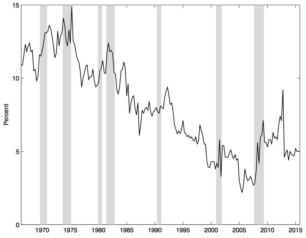
The start of the Great Recession marked a striking break in the behavior of the US
personal saving rate. After gradually declining over the previous 30 years, the saving
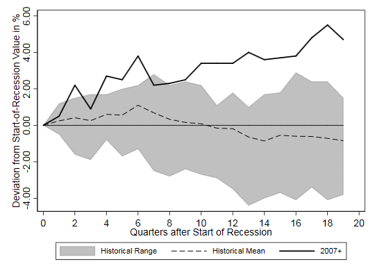
rate doubled during the recession (Figure 1(a)), and even 5 years later, exceeded
its pre-crisis level by 4 percentage points (Figure 1(b)). Surprising weakness of
consumption growth (relative to income growth) was a key element in explanations
of why, year after year, the recovery was weaker than forecasters expected. The
“secular stagnation” hypothesis of Summers (2013, 2015), Krugman (2013, 2014),
Gordon (2015), and others is the most provocative interpretation of these facts,
but even skeptics of secular stagnation have acknowledged that surprisingly weak
consumption growth played a role in the anemic recovery (Hamilton, Harris, Hatzius, and
West (2016)).
Standard consumption models incorporate several mechanisms that interact with
income dynamics to generate the saving rate; the channels that have received the
most attention include ‘wealth effects,’ the availability of credit, and precautionary
motives.
But we are not aware of any work that has attempted to quantify the relative importance of
these channels using the full (secular and cyclical) variation in the available historical data.
Our contribution is to use a simple structural model of saving to construct such a quantitative
decomposition. Specifically, we estimate a tractable ‘buffer stock saving’ model (an extended
version of Carroll and Toche (2009)) with explicit and transparent roles for the
three factors emphasized above (the wealth, credit, and precautionary channels).
The model’s key intuition is that, in the presence of income uncertainty, optimizing
households have a target ratio of wealth to permanent income that depends on the usual
theoretical considerations (the coefficient of relative prudence, see Kimball (1993);
time preference; etc.) and on two features that have been harder to incorporate into
analytical models: The degree of labor income uncertainty and the availability of
credit.
Over the historical period for which the necessary data are available, the structural model is
able to capture the bulk of the variation in the saving rate—with a fit better than 0.90 in the R2
sense.
We find a statistically significant and economically important role for all three explanatory
variables. The trend decline in saving between the mid-1970s and 2007 is explained by the
continual easing of credit availability during the period of gradual financial deregulation that
began in the Carter administration (see Woolley (2012) for the history) and extended to the
brink of the Great Recession. Our measure of credit supply (based on the Fed’s
Survey of Senior Loan Officers) shows a substantial tightening during the Great
Recession, the first sustained curtailment since the 1970s. But according to the model’s
estimates, a larger contributor to the sharp increase in the saving rate during the Great
Recession was the collapse in household wealth, with an increased precautionary motive
(proxied by a measure of consumers’ unemployment expectations) playing the next
most important role. We find that, contra Eggertsson and Krugman (2012) and
Guerrieri and Lorenzoni (2017), redit contraction as the least important of the three
factors.
The rest of the paper is organized as follows. Section 2 presents the structural model and its
mechanics. Section 3 briefly describes our data sources; section 4 presents the estimates of the
model and the empirical decomposition of the saving rate. Section 5 compares our
framework to the key competing frameworks for thinking about the saving rate; section 6
concludes.
2 Theory: Target Wealth and Credit Conditions
Here we introduce the model that we will later estimate, a simple representative-consumer
buffer-stock saving model derived from Carroll and Toche (2009) (henceforth CT). We extend
the CT model to incorporate unemployment insurance, which gives the model a mechanism to
capture changes in credit availability (because borrowing is assumed to be limited by the
minimum possible income available to repay it).
2.1 Essentials of the Tractable Model
Under most specifications of uncertainty, Constant Relative Risk Aversion utility interacts
with uncertainty in ways that rule out any transparent analytical formulation of the forces at
work. The assumption that makes the CT model tractable despite its use of CRRA utility is
that unemployment risk takes a particularly stark form: Employed consumers face a constant
probability ℧ of becoming unemployed, and, once unemployed, can never become employed
again. The sense in which the model is tractable is that there is a closed form solution for the
level of target wealth, and the full consumption function (though numerical) can
be constructed from the target almost instantaneously using a simple difference
equation.
CT show that for the special case of logarithmic utility, the target ‘market resources’ ratio
for an employed consumer (roughly, spendable wealth) is:
where γ is the growth rate of labor income, r is the interest rate and 𝜗 = − log β is the time
preference rate.
A “Growth Impatience Condition” guarantees that the expression (γ + 𝜗 −r) in the
denominator is strictly positive. Using this fact, the equation has intuitive implications: Target
wealth is higher (the consumer saves more) when
- The consumer is more patient (the time preference rate 𝜗 is lower)
- Unemployment risk ℧ is higher (inducing a stronger precautionary motive)
- Expected future income is lower (that is, γ −r is smaller)
2.2 Determinants of Target Wealth
We modify the CT model by adding an ‘unemployment insurance’ (UI) system that
relaxes the natural borrowing constraint. In the CT model, households accumulate
positive wealth to prevent zero consumption when they become unemployed. But,
in the model in this paper, employed households are willing to borrow, because
they know they will not starve even if they become unemployed; their consumption
function shifts to the left. However, such consumers will limit their indebtedness to an
amount small enough to guarantee that consumption will remain strictly positive
even if they become unemployed (so, it is the ‘natural borrowing constraint’ that
shifts).
The budget constraint depends on the consumer’s employment status. We denote with
lower-case m and c the levels of market resources M (market wealth plus current income) and
consumption C normalized by the corresponding period’s pretax labor income ℓW (the
product of individual labor productivity ℓ and the aggregate wage W); ℓW grows by Γ = 1 + γ
per period. Next period’s market resources ratio mt+1 is the sum of current market resources
mt net of consumption ct, augmented by the (growth-adjusted) interest factor R∕Γ and
income. For the employed consumer (normalized) after-tax labor income is 1 −τ, while for the
unemployed consumer the unemployment benefit is ς (both expressed as a fraction labor
income). The unemployment benefit ς is financed on a pay-as-you-go basis by a lump
sum tax τ. Under these assumptions the (normalized) dynamic budget constraint
is:
 | (2) |
Generalizing formula (1) for relative risk aversion ρ > 1 and allowing for UI benefits ς, the
employed consumer’s target market resources ratio me can be written as a function characterized
by:
 | (3) |
The target wealth me increases with unemployment risk ℧, as consumers build up a larger
precautionary buffer of savings. An easing of credit conditions (which we denote as
‘CEA’)—an increase in the CEA index (modelled as an increase in ς)—allows households to
borrow more and thus reduces the need to accumulate wealth for consumption smoothing. A
higher interest rate R increases the rewards to holding wealth and thus increases
the amount held. Faster expected growth of labor income Γ translates into a lower
wealth target because optimists consume more now in anticipation of their future
prosperity (the ‘human wealth effect’). Increasing risk aversion ρ raises target wealth
in a way that is qualitatively similar to the effects of an increase in uncertainty.
And of course, making the consumer more patient (increasing β) increases target
wealth.
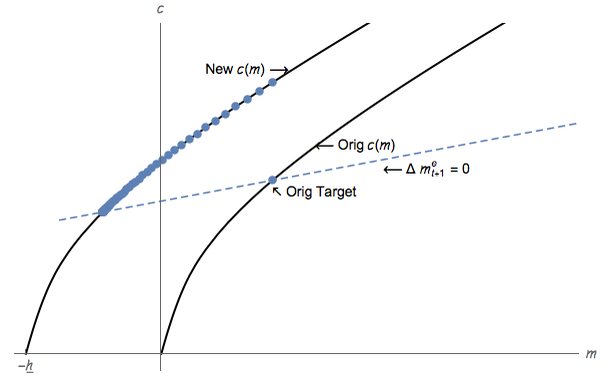
2.3 The Three Channels: A Graphical Exposition
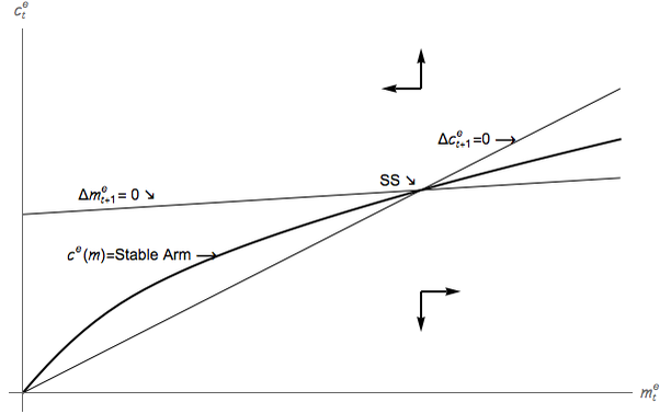
Figure 3a shows the phase diagram for the CT model. The (concave) consumption function
is indicated by the thick solid locus, which is the saddle path that leads to the steady
state (at which both consumption and market resources, c and m, are constant).
Because the precautionary motive diminishes as wealth rises, the model says the
saving rate is a declining function of market resources, an implication of consumption
concavity.
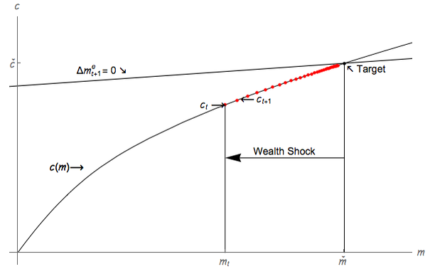
This consumption function can be used directly to analyze the effects of the three channels
affecting the saving rate. For a consumer who starts with market resources equal to the target,
mt = me, the consequences of a pure negative shock to wealth, depicted in Figure 3b, are
straightforward: Consumption declines upon impact, to a level below the value that would
leave m constant (the leftmost red dot); because consumption is below permanent income,
m (and thus c) rises over time back toward the original target (the sequence of
dots).
From an initial borrowing limit of 0 that requires wealth to be positive (m must be strictly
greater than c), an expansion of unemployment benefits results in a more generous natural
borrowing limit h (implying minimum net worth of −h < 0) and causes an immediate
increase in consumption for a given level of resources (Figure 3c). But over time, the
higher spending makes the consumer’s level of wealth decline, forcing a corresponding
gradual decline in consumption until wealth eventually settles at its new, lower target
level.
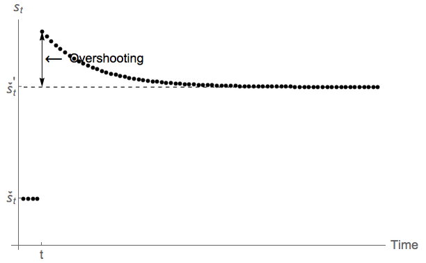
Figure 3d shows the consequences of a permanent increase in unemployment risk ℧ for the
dynamics of the personal saving rate (‘PSR’ henceforth), rather than the level of consumption
shown before. Qualitatively, the effects of a human-wealth-preserving spread in risk are
essentially the opposite of a credit loosening: On impact, the PSR jumps upward,
‘overshooting’ (cf. Dornbusch (1976)) the new target š′, followed by a gradual decline
toward š′ (which is higher than the original š). This nonmonotonic adjustment of saving to
shocks reflects the fact that, when target wealth rises, not only is a higher level of steady-state
saving needed to maintain higher target wealth, an immediate further boost to saving is
necessary to move from the current (inadequate) level of wealth up toward the new (higher)
target.
2.4 Comparison to Alternative ‘Structural’ Models
We use this simple, partial-equilibrium framework (instead of a richer but less tractable
HA-GE model) because our goal is to estimate a unified structural saving model whose “deep”
parameters are jointly identified using both business-cycle-frequency fluctuations AND
long-term trends. Both cyclical and secular changes in the saving rate have been large,
and a model that matched one set of facts (secular, or cyclical) but had strongly
counterfactual implications for the other would not be a satisfying description of
history.
We are not aware of prior papers that attempt this. Essentially all of the “structural”
literature has focused on cyclical dynamics, using one of two frameworks:
- Complex Heterogeneous Agent New Keynesian models (HANK) with serious
treatments of uncertainty
- Simple spender–saver Two-Agent New Keynesian models (TANK)
For the first class of models, the last decade or so has seen impressive progress in the
degree of realism achievable in the treatment of uncertainty, liquidity constraints, household
structure, and other first-order elements of households’ microeconomic environment. A
flourishing literature today explores the implications of these complexities for many questions;
see Krueger, Mitman, and Perri (2016) for a survey. However, at the current state of the art,
estimating such a model would be a considerable challenge, as estimation is generally
several orders of magnitude more computationally demanding than simulating a
calibrated version (which is what the existing literature has done). Furthermore, rich
microfounded models have usually been optimized for the specialized purposes of
examining in great depth a single question (such as the mechanisms of transmission of
monetary policy, Kaplan, Moll, and Violante (2016)) rather than, as we are attempting,
to address a number of different causal mechanisms, over different time horizons,
simultaneously. Finally, even if such a rich HA-GE model could be estimated, it is not clear
that the extra microeconomic realism would be worth the cost in transparency and
tractability.
Indeed, in advocating the use of TANK models, Debortoli and Galí (2017) argue that the
simplicity and transparency of models with only two agents more than make up for their lack
of fidelity to microeconomic facts. This point is reflected in the fact that, at present, central
banks and other entities that require a workhorse model for current analysis, have (to our
knowledge) not gone further than TANK models in their incorporation of heterogeneity.
Nonetheless, a major drawback of the TANK models is that they allow no role for
uncertainty either as an impulse or a propagation mechanism, despite the large
literature in recent years that has argued the uncertainty is a core element of business
cycle dynamics (see, e.g., cf. Bloom, Floetotto, Jaimovich, Saporta-Eksten, and
Terry (2018)).
Our model occupies a middle ground. We have only a single agent (making our model
simpler in one respect even than the TANK models), but that agent’s consumption function is
nonlinear (making it harder to analyze analytically). This nonlinearity brings a major benefit,
though, in providing a way to accommodate two mechanisms that do not meaningfully exist in
TANK models: Uncertainty and credit constraints. Furthermore, like a TANK model, its
parameters can be straightforwardly estimated to match targeted macroeconomic facts (in our
case, the saving rate).
Likely because of its tractability and simplicity, our model (as introduced in a draft version
of this paper) has been found useful as a tool to understand saving dynamics in a number of
countries in addition to the US. The model has been used explicitly to forecast
consumption and the saving rate at the Bank of England (Burgess, Fernandez-Corugedo,
Groth, Harrison, Monti, Theodoridis, and Waldron (2013)). Mody, Ohnsorge, and
Sandri (2012) use a version of it to motivate an empirical exercise which concludes that
labor income uncertainty contributed by at least two fifths to the increase in the
saving rate in advanced economies during the Great Recession (consistent with our
structural estimates below). Trichet (2010) argues (referring to our model) that the
precautionary motive contributed to the high saving rate in advanced economies after
2008.
2.4.1 Why We Do Not Endogenize Asset Prices
Arguably a deeper problem, both with our paper and with the other literature cited above, is
the choice to take as exogenous some of the variation that we would most urgently like to
understand. In particular, our model’s finding that a ‘wealth effect’ explains part of the
increase in saving in the Great Recession begs the question of what caused the asset price
movements that underlie the wealth effect (in stocks, housing and bonds). If, as seems likely,
an important driver of asset prices is the degree of uncertainty (cf. Bekaert, Engstrom, and
Xing (2009), Drechsler (2013)), then our method will substantially underestimate the
cyclical importance of uncertainty, attributing part of uncertainty’s true effect to
developments (asset prices; credit availability) that are themselves consequences of
uncertainty.
A vast literature has attempted to model asset pricing in general equilibrium. While some
progress has been made in understanding the cross-sectional heterogeneity of asset holdings
(cf. Gomes and Michaelides (2007)), for our purposes what is needed is a model that can
capture the cyclical and secular time series of returns. The extent to which no consensus exists
is highlighted by the diversity of the recent literature that has sought to endogenize the
precipitous decline of net worth and house prices during the Great Recession. In
this attempt, different authors have built into their models a number of alternative
mechanisms, including the presence of a exogenous but rare Great-Depression-like
state, exogenous shocks to expectations, or endogenous changes in illiquidity of
housing.
The existence of this literature suggests that no single model of asset pricing is adequate both
for “normal” times and for the Great Recession; more broadly, it seems fair to say that no
single asset pricing model has come to be viewed as robustly applicable to most times and
places, or for both high-frequency cyclical and low-frequency secular movements in asset
prices. If we were to incorporate any non-consensus model of asset pricing (and, at this point,
all asset-pricing models are non-consensus models), our paper would inevitably (and correctly)
judged to be more about the performance of that asset pricing model than anything
else.
The exogeneity assumptions bring us to a final reason for using our tractable model, which
is that a central purpose of this paper has been to bring to light the existence of some
surprisingly simple empirical relationships between the saving rate and our three explanatory
variables. The construction of an elaborate model that required many pages to set up and
explain, and many more pages to estimate, might have drawn attention away from the
simplicity of the empirical foundations of the paper, in which the key results are evident even
in the OLS reduced form estimates. Our penultimate section 5 examines the empirical
performance of our model in comparison with a number of alternatives (including the
reduced form model) and argues that our structural model has advantages over any of
them.
3 Data and Measurement Issues
This section describes how we measure our key variables (shown in Figure 4).
The saving rate is from the BEA’s National Income and Product Accounts and is expressed
as a percentage of disposable income.
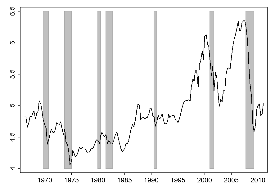
Motivated by equation (2), we measure household’s normalized market resources mt as 1
plus the ratio of household net worth to disposable income (Figure 5a). For net worth we use
data from the Federal Reserve’s Financial Accounts; this variable is lagged by one quarter
to account for the fact that data on net worth are reported as the end-of-period
values.
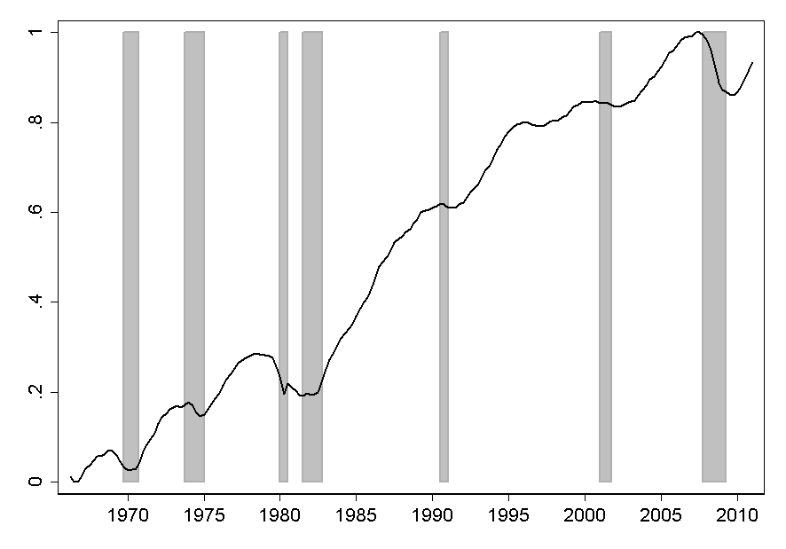
Our measure of credit availability, which we call the ‘Credit Easing Accumulated’ index
(CEA; Figure 5b) is adapted from work by John Muellbauer and various coauthors
(Muellbauer (2007), Duca, Muellbauer, and Murphy (2010) and Aron, Duca, Muellbauer,
Murata, and Murphy (2011); for a related approach, see Hall (2011)). It is constructed using
a question from the Federal Reserve’s Senior Loan Officer Opinion Survey (SLOOS) on Bank
Lending Practices. The question asks about banks’ willingness to make consumer installment
loans now as opposed to three months ago. To calculate a proxy for the level of credit
conditions, the scores from the survey were accumulated, weighting the responses by the
contemporaneous debt-to-income ratio to account for the increasing trend in that variable,
and normalizing the result to range between 0 and 1 to make the interpretation of regression
coefficients straightforward. We use the question on installment loans because it
is available since 1966; other measures of credit availability, such as for mortgage
lending, move closely with the index on consumer installment loans over the sample
period when both are available until 2008. While the two indices diverge in the
Great Recession and afterward, this corresponds to the period when there was a
massive shift of mortgage origination from banks (the respondents to the SLOOS)
to government sponsored entities (Fannie Mae, Freddie Mac, and others). That
shift brings into question the continued relevance of the direct SLOOS index of
mortgage lending conditions. There was no similar profound institutional change
in the market for installment lending, which is one reason it might reasonably be
interpreted as a consistent indicator of the overall credit environment (given its
high correlation with other credit supply indices in the period before the Great
Recession).
The CEA index is taken to measure the availability/supply of credit to a typical household
as it is affected by factors other than the level of interest rates—for example, through
constraints on loan-to-value or loan-to-income ratios, availability of mortgage equity
withdrawal and mortgage refinancing. The broad trends in the CEA index seem to reflect well
the key developments of the US financial market institutions, which we summarize as follows:
Until financial deregulation began in the late 1970s, consumer lending markets were heavily
regulated and segmented. After the phaseout of interest rate controls beginning in the
early 1980s, the markets became more competitive, spurring financial innovations
that led to greater access to credit. Technological progress leading to new financial
instruments and better credit screening methods (Pagano and Jappelli (1993)), a greater
role of nonbanking financial institutions, and the increased use of securitization all
contributed to the dramatic rise in credit availability from the early 1980s until
the onset of the Great Recession in 2007, at which point a substantial drop in the
CEA index was associated with the funding difficulties and de-leveraging of financial
institutions.
We measure a proxy 𝔼 tut+4 for unemployment risk ℧t using re-scaled answers to the
question about the expected change in unemployment in the Thomson Reuters/University of
Michigan Surveys of Consumers. In particular, we estimate 𝔼 tut+4 using fitted values
Δ4ût+4 from the regression of the four-quarter-ahead change in unemployment rate
Δ4ut+4 ≡ ut+4 − ut on the answer in the survey, summarized with the balance statistic
UExptBS:
The coefficient α1 is highly statistically significant, indicating that households do have
substantial information about the direction of future changes in the unemployment rate. As
expected, our 𝔼 tut+4 series is strongly correlated with unemployment rate and predicts its
dynamics (Figure 5c).
Data for our empirical measure of credit conditions are available starting 1966q2, and the data
we use in estimation cover that date to 2011q4.
We do not use data after 2011 for several reasons. First, personal saving rate statistics are
subject to large revisions until some five years after the first data release (after the BEA receives
much higher quality personal income data from the IRS). To quote Nakamura and Stark (2007):
“[M]uch of the initial variation in the personal saving rate across time was meaningless
noise.”
As their paper documents, it is not uncommon for the saving rate to be revised by 3–5 percent
of disposable income after several benchmark revisions.
Second, our index of credit availability is increasingly questionable after 2011 because of the
apparent divergence in credit conditions for installment and mortgage loans: Various sources
(including the Mortgage Credit Availability Index of the Mortgage Bankers’ Association; see
also Bhutta (2015)) document continued tight credit conditions after 2011. If, as this work
suggests, mortgage credit remained tighter than indicated by our installment loans index after
2012, that could explain part of the continued high saving rate in the post-2012 period, which
would be mispredicted by a mismeasured credit conditions index. Alternatively, saving
attitudes may have changed after the Great Recession due to the substantial shock of the
Great Recession, perhaps because of “scarring” effects (see, e.g., Malmendier and Shen (2018),
Jordà, Schularick, and Taylor (2015), Hall (2012)); for evidence that financial crises have
much longer-lasting effects than usual business cycle fluctuations, see Reinhart and
Rogoff (2009). All of these are reasons to worry about data from the post-Great-Recession
period.
4 Structural Estimation
This section estimates the structural model of section 2 by minimizing the distance between
the saving rate implied by the model and its empirical counterpart.
4.1 Estimation Procedure
In more detail, the structural estimation proceeds as follows. We assume that households
observe exogenous movements in unemployment risk ℧ and credit availability
h, and
that there are simple mappings from our credit availability index CEAt to the location of the
consumers’ borrowing constraint ht and from measured unemployment expectations 𝔼 tut+4 to
℧t:
Collecting the parameters Θ = {β,𝜃CEA,𝜃℧,𝜃u}, and the time-t observable variables as
zt = {mt, CEAt, 𝔼 tut+4}, the model implies a “saving rate function” s(zt; Θ) which we aim to
compare to the saving rates observed in the data, stmeas. Our objective is therefore to find the
parameter vector Θ that minimizes the distance between actual saving rates and those implied
by the model:
 | (5) |
Minimization of (5) is a non-linear least squares problem for which the standard asymptotic
results apply. The estimates have the asymptotic normal distribution:
 where the variance matrix can consistently be estimated with
 for
σ2 =
for
σ2 =  ∑
t=1T
∑
t=1T  s
tmeas − s(zt; Θ)
s
tmeas − s(zt; Θ) 2 and the T × 4 gradient matrix of the saving rate function
F = ∇Θ′s(zt; Θ) evaluated at Θ (which is calculated numerically).
2 and the T × 4 gradient matrix of the saving rate function
F = ∇Θ′s(zt; Θ) evaluated at Θ (which is calculated numerically).
4.2 Estimates and the Model Fit
Table 1 presents the estimation results. The calibrated parameters—the quarterly real interest
rate r = 0.04∕4, quarterly wage growth ΔW = 0.01∕4 and the coefficient of relative risk
aversion ρ = 2—are conventional and meet (together with the estimated discount factor β) the
conditions sufficient for the problem to have a well-defined solution (see Carroll and
Toche (2009)).
The estimated quarterly discount factor β = 1 − 0.0065 = 0.9935, or 0.974 at an annual
frequency, lies in the standard range. As for the horizontal shift in the consumption function
ht driven by credit availability, the estimates of the scaling factor 𝜃CEA implies that ht varies
between 0 and 8.89∕4 ≈ 2.2, implying that financial deregulation resulted at its peak in an
availability of credit in 2007 that was greater than credit availability at the beginning of
our sample in 1966 by an amount equal to about 220 percent of annual income
(for an average household)—not an unreasonable figure given the now-prevailing
rule of thumb that homebuyers can afford a house costing three times their annual
income.
The estimated intensity of perceived unemployment risk reflects that fact that the risk in
our setup is purely permanent: the estimated risk ℧t ranges between 1.25 × 10⁻⁴ and
1.5 × 10⁻⁴ per quarter. The peak magnitude of ℧
t (of 1.5 × 10⁻⁴) implies that over the life
cycle of 50 years or 200 quarters, the workers face a probability of roughly 3 percent to
become (permanently) unemployed. Given the average aggregate unemployment rate of
roughly 6 percent in our sample and given that much of this risk is in reality transitory, the
estimated scaling of ℧t seems broadly plausible. The estimated risk ℧t is highly
counter-cyclical, reflecting movements in the unemployment rate, further magnified by
unemployment expectations.
The quantitative interpretation of the coefficients in the model can be summarized by
calculating that a 20 percent increase in uncertainty (not out of line for a recession) results in
a roughly 1-percentage-point increase in the saving rate. A way to judge the plausibility of this
prediction is to consider a similar increase in uncertainty in a microeconomically richer model,
such as Carroll, Slacalek, Tokuoka, and White (2017). A 20 percent increase in the variance of
permanent shocks in that model predicts a similar increase in the saving rate, as that implied
by our estimates above.
4.3 What Drives the Saving Rate? A Decomposition
Time-variation in the fitted saving rate arises as a result of movements in its three
time-varying determinants: wealth, uncertainty and credit conditions; Figure 6.
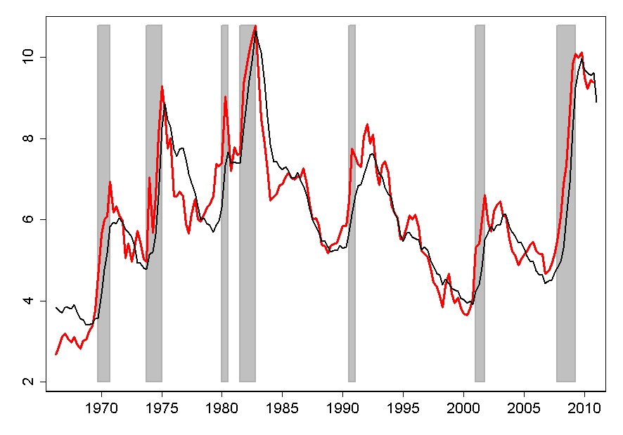
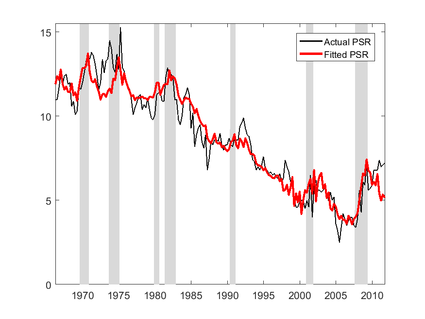
Overall, the estimated structural model provides a good explanation for both low-frequency
and business-cycle variation in the saving rate (red line in Figure 7a). The model matches
both the 30-year decline in the saving rate before 2007 and the cyclical increases in saving
during recessions. For the Great Recession, Table 2 shows that the model implies an increase
in the saving rate of about 2.6 percentage points between the 2006–2007 period (immediately
before the GR) and the 2009–2010 period (skipping the transitional year of 2008). This
matches exactly the 2.6 point measured change in the saving rate. Of that 2.6 point change,
the drop in wealth accounts for about half, with the increase in uncertainty accounting for a
bit more of the remainder than the decrease in credit. (Recall also our earlier point
that this decomposition understates the full role of uncertainty, if the drop in asset
prices or the tightening of credit were themselves partly the result of increases in
uncertainty).
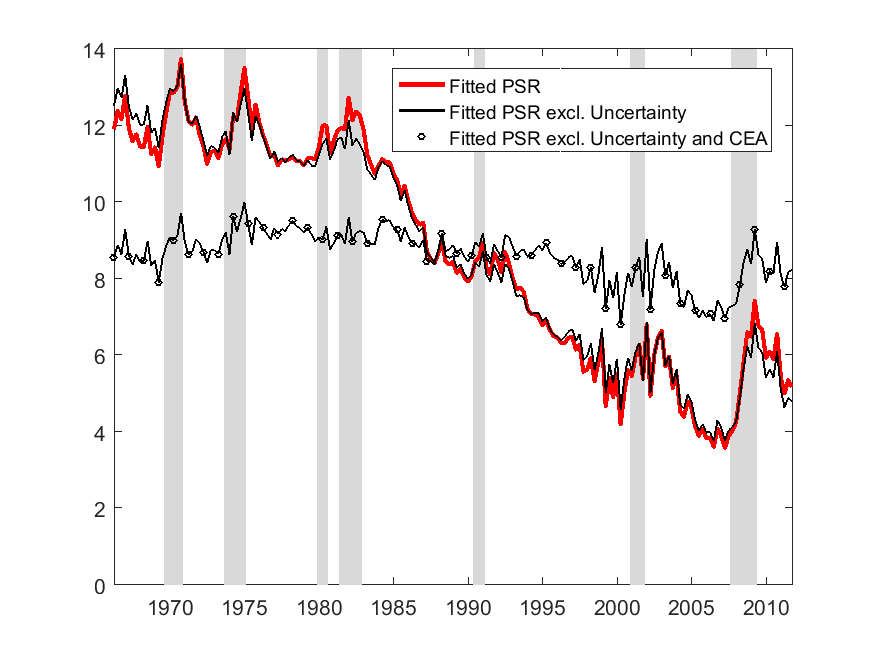
To gauge the relative importance of the three variables over the full sample, we
sequentially switch off the channels by setting the series equal to their sample
means.
The main takeaway is that the CEA is essential in capturing the trend decline in the PSR
between the 1980s and the early 2000s. The wealth fluctuations contribute to a good
fit of the model at the business-cycle frequencies, and the cyclical fluctuations in
uncertainty magnify the increases in the PSR during recessions, including in the Great
Recession.
The implied estimates of the wealth effect on consumption are on the low end of the range
produced by existing empirical estimates, which lie between 0.02–0.07 (Carroll, Otsuka, and
Slacalek (2011), Mian, Rao, and Sufi (2011), Berger, Guerrieri, Lorenzoni, and
Vavra (2018) and many others). For example, during the Great Recession, of the
5-percentage-point increase in the saving rate the model (black circled line in Figure 7b)
ascribes roughly 3 percentage points to the drop in net worth, which amounted to
roughly 200 percent of disposable income (Figure 5a), implying a marginal propensity
consume out of wealth (MPCW) of 3∕200 = 0.015. The key reason for this contrast is
that our structural estimates attribute a substantial role to uncertainty and credit
conditions. This finding suggests that much of what has been interpreted as pure “wealth
effects” in the prior literature may actually have reflected precautionary or credit
availability effects that are correlated with wealth (a result in line with much of the
household-level evidence, including Hurst and Stafford (2004), Cooper (2013), Aruoba, Elul,
and Kalemli-Ozcan (2019) and others, who stress the role of credit availability and
collateral constraints). (This explanation is supported by our reduced form results in
section 5.3, in which the coefficient on wealth in the saving rate equation is substantially
higher in the univariate regression, than when controlling for uncertainty and credit
conditions.)
Finally, our simple model does not adequately account for household heterogeneity. In a
model like that of Carroll, Slacalek, Tokuoka, and White (2017), wealth shocks mostly hit
wealthy people who have low MPCs, while income shocks (like stimulus checks) hit the whole
population which includes many low-wealth people who have high MPCs. If this is the right
explanation, an RA model (ours included) is by its fundamental nature incapable of
reconciling the conflict. In addition, a substantial proportion of shocks to net worth are
driven by housing wealth, for which evidence suggests that the MPC is likely lower
than for liquid assets (including increases from income tax rebates; for a compelling
quasi-natural experiment on the size of housing wealth effects, see Kessel, Tyrefors, and
Vestman (2019)).
5 Empirical Evaluation of Alternative Models
Here we argue that our model has advantages over the chief alternatives that can be readily
evaluated.
5.1 Quadratic Utility
Since Hall (1978), an optimizing model with quadratic utility has been an influential
benchmark for aggregate consumption dynamics (especially once one understands that
linearized DSGE models are basically indistinguishable from the Hall model). The key
distinction from our theoretical model in section 2 is that, in contrast to CRRA utility, under
quadratic utility uncertainty has no effect on consumption dynamics; quadratic-utility
households do not engage in precautionary saving and do not have a wealth target (other than
the current level of wealth).
The model without uncertainty turns out to be distinctly inferior to our buffer stock saving
model. We have already seen above in Table 1 that the intercept 𝜃℧ and the sensitivity to
uncertainty 𝜃u enter very significantly the unemployment risk equation (4) of the structural
model. This evidence is confirmed in a reduced form linear regression estimation,
where business-cycle variation in labor market uncertainty is strongly related to
the PSR, both on its own and controlling for other variables (columns 1 and 3 of
Table 3, respectively). The results imply that a 1 percentage point increase in
expected unemployment rate increases the saving rate by roughly 0.2–0.6 percentage
points.
These results confirm a large body of complementary evidence on how uncertainty affects
aggregate consumption and saving going back to 1990s. Recently, the evidence based on
household-level data has shown that uncertainty is also important for macroeconomic
outcomes (Bloom, Floetotto, Jaimovich, Saporta-Eksten, and Terry (2018), Kaplan and
Violante (2018) and many others). These findings, mostly based on ‘normal’ (shallow)
recessions, were further strengthened during the Great Recession when (according to Krueger,
Mitman, and Perri (2016) and the references in footnote 8) uncertainty amplified the drop in
house prices, employment and consumption.
5.2 Demographics and Saving
A long tradition of work, stemming from the seminal work of Modigliani and
Brumberg (1954), examines the implications of demographic change for saving using
calibrations and simulations of various life-cycle models (usually in an OLG setup).
Overall, this strand of work has concluded that at the higher frequencies (e.g., annual)
demographic changes do not substantially affect changes in saving because they are both
small and very slow-moving (Summers and Carroll (1987), Parker (2000) and many
others).
If demographic trends could provide a compelling explanation for the long-term decline in
the saving rate leading up to 2007, that might constitute a plausible alternative to our story
based on increased credit availability in the era of financial deregulation. But Auerbach, Cai,
and Kotlikoff (1991) and related papers argued persuasively in the early 1990s that the
first-order implication of demographics was that there should be a sustained rise in the
saving rate for many years until the baby boom generation hit its peak earnings
years around 2000–2005, and a declining saving rate thereafter. This is precisely
the opposite of the actual pattern (the baby boom generation began exiting the
“high-saving” phase of life and entering the supposedly “low-saving” retirement
phase during exactly the interval when the saving rate stopped declining and then
rose).
This point is roughly captured in Figure 9a which plots the old-age dependency ratio,
which began rising faster around 2010 when large numbers of baby boomers began reaching
retirement age. In Table 3, column 2 we estimate that the coefficient on the old-age
dependency ratio is negative, which would suggest that the increase in the share of
people older than 65 years should have reduced the saving rate, so the correlations go
the wrong way for a demographic story (confirming the large prior literature after
Auerbach, Cai, and Kotlikoff (1991) that failed to find meaningful demographic
effects).
5.3 Reduced-Form vs Structural Models of Saving
We now ask to what extent the main features of the structural model of section 2 can be
summarized in a simple reduced-form linear regression:
 | (6) |
This specification can be readily estimated using OLS estimators (Table 3, column 3) and,
at a minimum, can be interpreted as summarizing basic stylized facts about the
data.
We have mentioned (in section 5.1) that the estimates of the “Baseline” model (6) are
significant and explain more than 90 percent of variation in the saving rate. As expected from
the structural model, the point estimates indicate a strong negative correlation of saving with
net wealth and credit conditions, and a positive correlation with unemployment
risk.
The coefficient on the Credit Easing Accumulated index is highly statistically significant
with a t-statistic of more than 14. (Of course, this t-statistic should be taken with a several
grains of salt given the obvious trends in both variables, and the cautionary literature about
regressions of trends on trends; but aside from demographics (which go the wrong way), there
are no other variables that are core constituents of standard saving models that
have had powerful trends like this, so the case for spurious correlation is weaker
than it sometimes is). The point estimate of γCEA implies that increased access to
credit over the sample period until the Great Recession reduced the PSR by about
8 percentage points of disposable income. In the aftermath of the Recession, the
CEA index declined between 2007 and 2010 by roughly 0.11 as credit supply tightened,
contributing roughly 0.64 percentage point to the increase in the saving rate. Finally,
once the three variables are included jointly, the time trend ceases to be significant
(column 4).
Given how well the baseline linear reduced-form model captures the saving rate, one might
wonder what value is added by construction of the structural model we proposed earlier. A
first point to make here is that when we simulate the estimated version of our model
and perform linear regressions on the corresponding generated data, the result is
very close to being linear (the R2 is 0.975). Essentially, therefore, the difference
between the two approaches is that the OLS regression puts no restrictions at all
on the linear relationships between the variables, while the structural estimation
puts stringent requirements that those linear relationships be tightly constrained to
the small subset of nearly linear relationships that is a good approximation to the
structural theory. The fact that the R2 from the structural estimation is essentially the
same as for the unrestricted model (both of them round to 0.91) was by no means
inevitable and indicates that the structure imposed by the model does no violence to the
data.
5.3.1 Why Estimate a Structural Model When OLS Works Fine?
Because structural estimation restricts empirical relationships to those that are compatible
with a theory, structural models by their intrinsic nature fit the data worse than an
unrestricted data-fitting exercise; the advantages of structural modeling (articulated below)
can nevertheless make such estimation worth the sacrifice in data-fitting ability. In
the case at hand, however, the structural model fits the data nearly as well as an
unrestricted OLS regression. Thus, in our context, the case for structural modeling is
stronger than in the usual case where there is a significant penalty in data-fitting
ability.
Some of the advantages of having a structural model are:
- If the structure imposed is one that has considerable backing from other contexts
or kinds of data, it is less likely that the fit of the model to the data is spurious
(in the sense of failing to capture any reliable or causal economic relationship).
- The structural model can provide insights that could not be obtained from
the reduced form model. For example, the “overshooting” result implied by the
structural model might have important consequences for business cycle dynamics
even if the fit of the structure that embodies those dynamics is statistically inferior
to the reduced form fit.
- The structural model has implications for ways to test the ideas using data other
than those on which it was estimated. In this case, for example, the structural
model would suggest that it would be useful to look at regional or local data in
which the endogeneity of aggregate asset prices and credit conditions could be
controlled for by looking at differences in unemployment expectations and saving
responses across regions in an aggregate economy where most of the movements
in the other explanatory variables are not region-specific.
5.4 Further Robustness Checks
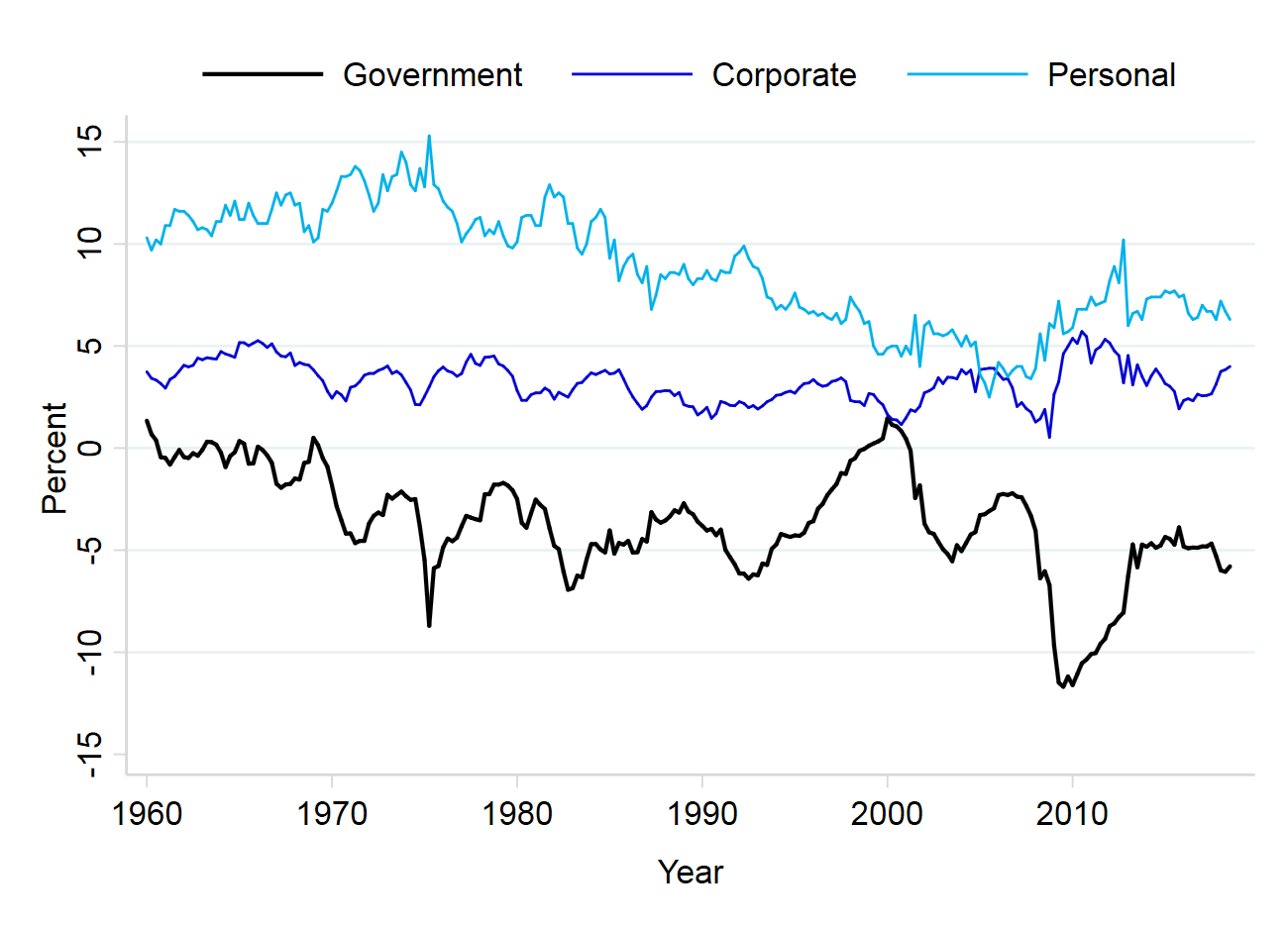
Columns 5 and 6 of Table 3 summarize the correlations of the personal saving rate with two
variables that some theories suggest might be related to it: government saving (Figure 9b)
and income inequality (Figure 9c).
Column 5 reports that there is indeed a negative correlation between government and
personal saving, though the size of the coefficient, −0.15, implies only a modest crowding out.
More than a support for the Ricardian equivalence—the hypothesis that households
observing higher government saving should save less themselves (as they should expect
lower taxes in the future)—the finding seems to reflect reverse causality between
private and public saving, the fact that during recessions government saving falls
(e.g., due to higher outlays on unemployment insurance), while personal saving rises
for precautionary reasons (see work of Elmendorf and Mankiw (1999) and many
others).
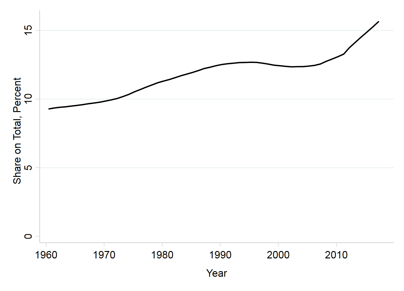
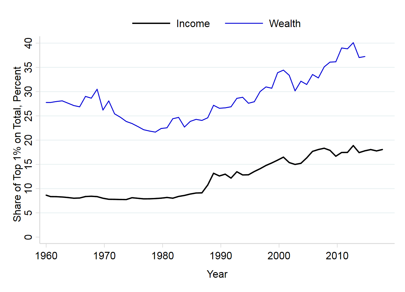
Finally, in column 6 we evaluate whether growing income inequality (shown in Figure 9c)
has resulted in an increase in the aggregate saving rate: Microeconomic evidence points to
high personal saving rates among the higher-permanent-income households (Carroll (2000);
Dynan, Skinner, and Zeldes (2004)), whose share on total income has been rising. Having
experimented with numerous measures of the top shares of Piketty and Saez (2003), we find
little evidence of a substantial and statistically significant correlation between saving and
income inequality.
6 Conclusions
We show that a simple representative-consumer model of buffer stock saving can match most
of the time-series variation in the aggregate US personal saving rate over the past 50 years. In
the model, saving depends on the gap between the ‘target’ and actual wealth, with the target
determined by credit availability and uncertainty.
We estimate that these three factors—credit availability, shocks to household wealth, and
movements in income uncertainty proxied by unemployment risk—have all been important in
driving the saving rate. In particular, the relentless expansion of credit supply between the
early-1980s and 2007 (likely largely reflecting financial innovation and liberalization), along
with higher asset values and consequent increases in net wealth (possibly also partly
attributable to the credit boom) encouraged households to save less out of their disposable
income. At the same time, the fluctuations in wealth and labor income uncertainty, for
instance during and after the burst of the information technology and credit bubbles
of 2001 and 2007, can explain the bulk of business cycle fluctuations in personal
saving.
The model we estimate could be extended to analyze the implications of the ‘overshooting’
of saving in response to business-cycle shocks. For example, the model suggests that in a
recession an optimizing government might want to counteract the part of the consumption
decline that reflects overshooting. In an economy rendered non-Ricardian by liquidity
constraints and/or uncertainty, the existence of precautionary saving thus provides a potential
rationale for counter-cyclical fiscal policy.
More generally, the simple buffer stock saving model we estimate could provide insights into
the current debate about the role household heterogeneity for macroeconomic outcomes. The
model is both easy to solve and provides a setup to meaningfully analyze the effects on
uncertainty on the macro-economy. Consequently, the model could be a useful middle ground
between a setup with a realistic but complex description of household heterogeneity (HANK)
and a simple two-agent spender–saver setup (TANK) that cannot accommodate roles for
credit availability or uncertainty.
References
Abiad, Abdul, Enrica Detragiache, and Thierry Tressel (2010): “A New
Database of Financial Reforms,” IMF Staff Papers, 57(2), 281–302.
Aron, Janine, John V. Duca, John Muellbauer, Keiko Murata, and Anthony
Murphy (2011): “Credit, Housing Collateral, and Consumption: Evidence from Japan, the
U.K., and the U.S.,” Review of Income and Wealth.
Aruoba, S Boragan, Ronel Elul, and Sebnem Kalemli-Ozcan (2019): “How Big
is the Wealth Effect? Decomposing the Response of Consumption to House Prices,” FRB of
Philadelphia Working Paper.
Auerbach, Alan J., Jinyong Cai, and Laurence J. Kotlikoff (1991): “U.S.
Demographics and Saving: Predictions of Three Saving Models,” Carnegie–Rochester
Conference Series on Public Policy, 34(1), 135–156.
Baker, Scott R, Nicholas Bloom, and Steven J Davis (2016): “Measuring
economic policy uncertainty,” The Quarterly Journal of Economics, 131(4), 1593–1636.
Bekaert, Geert, Eric Engstrom, and Yuhang Xing (2009): “Risk, uncertainty, and
asset prices,” Journal of Financial Economics, 91(1), 59–82.
Berger, David, Veronica Guerrieri, Guido Lorenzoni, and Joseph Vavra
(2018): “House Prices and Consumer Spending,” Review of Economic Studies, 85(3),
1502–1542.
Bhutta, Neil (2015): “The Ins and Outs of Mortgage Debt During the Housing Boom
and Bust,” Journal of Monetary Economics, 76(C), 284–298.
Bloom, David E., David Canning, Richard K. Mansfield, and Michael Moore
(2007): “Demographic Change, Social Security Systems and Savings,” Journal of Monetary
Economics, 54, 92–114.
Bloom, Nicholas, Max Floetotto, Nir Jaimovich, Itay Saporta-Eksten, and
Stephen J. Terry (2018): “Really Uncertain Business Cycles,” Econometrica, 86(3),
1031–1065.
Bosworth, Barry, and Gabriel Chodorow-Reich (2007): “Saving and Demographic
Change: The Global Dimension,” working paper 2, Center for Retirement Research, Boston
College.
Burgess, Stephen, Emilio Fernandez-Corugedo, Charlotta Groth, Richard
Harrison, Francesca Monti, Konstantinos Theodoridis, and Matt Waldron
(2013): “The Bank of England’s Forecasting Platform: COMPASS, MAPS, EASE and the
Suite of Models,” working paper 471, Bank of England.
Carroll, Christopher D. (1992): “The Buffer-Stock Theory of Saving: Some
Macroeconomic Evidence,” Brookings Papers on Economic Activity, 1992(2), 61–156,
http://econ.jhu.edu/people/ccarroll/BufferStockBPEA.pdf.
__________ (2000): “Why Do the Rich Save So Much?,” in Does Atlas Shrug? The Economic
Consequences of Taxing the Rich, ed. by Joel B. Slemrod. Harvard University Press,
http://econ.jhu.edu/people/ccarroll/Why.pdf.
__________ (2001): “A Theory of the Consumption Function,
With and Without Liquidity Constraints,” Journal of Economic Perspectives, 15(3), 23–46,
http://econ.jhu.edu/people/ccarroll/ATheoryv3JEP.pdf.
Carroll, Christopher D., and Olivier Jeanne (2009): “A Tractable Model of
Precautionary Reserves, Net Foreign Assets, or Sovereign Wealth Funds,” NBER Working
Paper Number 15228, http://econ.jhu.edu/people/ccarroll/papers/cjSOE.
Carroll, Christopher D., Misuzu Otsuka, and Jiri Slacalek (2011): “How Large
Are Financial and
Housing Wealth Effects? A New Approach,” Journal of Money, Credit, and Banking, 43(1),
55–79, http://econ.jhu.edu/people/ccarroll/papers/cosWealthEffects/.
Carroll, Christopher D.,
Jiri Slacalek, Kiichi Tokuoka, and Matthew N. White (2017): “The Distribution
of Wealth and the Marginal Propensity to Consume,” Quantitative Economics, 8, 977–1020,
At http://econ.jhu.edu/people/ccarroll/papers/cstwMPC.
Carroll, Christopher D., and Patrick Toche
(2009): “A Tractable Model of Buffer Stock Saving,” NBER Working Paper Number 15265,
http://econ.jhu.edu/people/ccarroll/papers/ctDiscrete.
Cooper, Daniel (2013): “House Price Fluctuations: The Role of Housing Wealth as
Borrowing Collateral,” The Review of Economics and Statistics, 95(4), 1183–1197.
Curtis, Chadwick C., Steven Lugauer, and Nelson C. Mark (2015):
“Demographic Patterns and Household Saving in China,” American Economic Journal:
Macroeconomics, 7(2), 58–94.
Debortoli, Davide, and Jordi Galí (2017): “Monetary policy with heterogeneous
agents: Insights from TANK models,” Manuscript.
Demyanyk, Yuliya, Charlotte Ostergaard, and Bent E. Sørensen (2007): “U.S.
Banking Deregulation, Small Businesses, and Interstate Insurance of Personal Income,”
Journal of Finance, 62(6), 2763–2801.
Dornbusch, Rudiger (1976): “Expectations and Exchange Rate Dynamics,” Journal of
Political Economy, 84(6), 1161–1176.
Drechsler, Itamar (2013): “Uncertainty, time-varying fear, and asset prices,” The
Journal of Finance, 68(5), 1843–1889.
Duca, John V., John Muellbauer, and Anthony Murphy (2010): “Credit Market
Architecture and the Boom and Bust in the U.S. Consumption,” mimeo, University of
Oxford.
Dynan, Karen E., Jonathan Skinner, and Stephen P. Zeldes (2004): “Do the
Rich Save More?,” Journal of Political Economy, 112(2), 397–444.
Eggertsson, Gauti B., and Paul Krugman (2012): “Debt, Deleveraging, and the
Liquidity Trap: A Fisher–Minsky–Koo Approach,” The Quarterly Journal of Economics,
127(3), 1469–1513.
Elmendorf, Douglas, and N. Gregory Mankiw (1999): “Government Debt,” in
Handbook of Macroeconomics, ed. by J. B. Taylor, and M. Woodford, vol. 1, Part C,
chap. 25, pp. 1615–1669. Elsevier, 1 edn.
Favilukis, Jack, Sydney C. Ludvigson, and Stijn Van Nieuwerburgh (2017):
“The Macroeconomic Effects of Housing Wealth, Housing Finance, and Limited Risk Sharing
in General Equilibrium,” Journal of Political Economy, 125(1), 140–223.
Garriga, Carlos, and Aaron Hedlund (2018): “Housing Finance, Boom–Bust
Episodes, and Macroeconomic Fragility,” mimeo, University of Missouri.
Glover, Andrew, Jonathan Heathcote, Dirk Krueger, and José-Víctor
Ríos-Rull (2017): “Intergenerational Redistribution in the Great Recession,”
updated version of working paper 16924, National Bureau of Economic Research,
https://www.sas.upenn.edu/~dkrueger/research/RecessionNew.pdf.
Gomes, Francisco, and Alexander Michaelides (2007): “Asset pricing with limited
risk sharing and heterogeneous agents,” The Review of Financial Studies, 21(1), 415–448.
Gordon, Robert J (2015): “Secular stagnation: A supply-side view,” American
Economic Review, 105(5), 54–59.
Gorea, Denis, and Virgiliu Midrigan (2018): “Liquidity Constraints in the U.S.
Housing Market,” mimeo, New York University.
Guerrieri, Veronica, and Guido Lorenzoni (2017): “Credit crises, precautionary
savings, and the liquidity trap,” The Quarterly Journal of Economics, 132(3), 1427–1467.
Hall, Robert E. (1978): “Stochastic Implications of the Life-Cycle/Permanent Income
Hypothesis: Theory and Evidence,” Journal of Political Economy, 96, 971–87, Available at
http://www.stanford.edu/~rehall/Stochastic-JPE-Dec-1978.pdf.
__________ (2011): “The Long Slump,” AEA Presidential Address, ASSA Meetings, Denver.
__________ (2012): “Quantifying the Forces Leading to the Collapse of GDP after the
Financial Crisis,” Manuscript, Stanford University.
Hamilton, James D, Ethan S Harris, Jan Hatzius, and Kenneth D West
(2016): “The equilibrium real funds rate: Past, present, and future,” IMF Economic Review,
64(4), 660–707.
Hubmer, Joachim, Per Krusell, and Anthony A. Smith, Jr. (2018): “A
Comprehensive Quantitative Theory of the U.S. Wealth Distribution,” mimeo, Yale
University.
Huo, Zhen, and José-Víctor Ríos-Rull (2016): “Financial Frictions, Asset
Prices, and the Great Recession,” Staff Report 526, Federal Reserve Bank of Minneapolis.
Hurst, Erik, and Frank Stafford (2004): “Home Is Where the Equity Is: Mortgage
Refinancing and Household Consumption,” Journal of Money, Credit and Banking, 36(6),
985–1014.
Imrohoroglu, Ayse, and Kai Zhao (2018): “The Chinese Saving Rate: Long-Term
Care Risks, Family Insurance, and Demographics,” Journal of Monetary Economics, 96(C),
33–52.
Jordà, Òscar, Moritz Schularick, and Alan M. Taylor (2015): “Leveraged
Bubbles,” Journal of Monetary Economics, 76(S), 1–20.
Justiniano, Alejandro, Giorgio Primiceri, and
Andrea Tambalotti (forthcoming): “Credit Supply and the Housing Boom,” Journal of
Political Economy.
Kaplan, Greg, Kurt Mitman, and Giovanni L. Violante (2017): “The Housing
Boom and Bust: Model Meets Evidence,” working paper 23694, National Bureau of Economic
Research.
Kaplan, Greg, Benjamin Moll, and Giovanni L. Violante (2016): “Monetary
Policy According to HANK,” Working Paper 21897, National Bureau of Economic Research.
Kaplan, Greg, and Giovanni L. Violante (2018): “Microeconomic Heterogeneity and
Macroeconomic Shocks,” Journal of Economic Perspectives, 32(3), 167–194.
Kessel, Dany, Björn Tyrefors, and Roine Vestman (2019): “The Housing Wealth
Effect: Quasi-Experimental Evidence,” Available at SSRN.
Kimball, Miles S. (1993): “Standard Risk Aversion,” Econometrica, 61(3), 589–611.
Krueger, Dirk, Kurt Mitman, and Fabrizio Perri (2016): “Macroeconomics and
Household Heterogeneity,” Handbook of Macroeconomics, 2, 843–921.
Krugman, Paul (2013): “Secular stagnation, coalmines, bubbles, and Larry Summers,”
New York Times, 16, 2013.
__________ (2014): “Four observations on secular stagnation,” Secular stagnation: Facts,
causes and cures, pp. 61–68.
Landvoigt, Tim (2017): “Housing Demand During the Boom: The Role of Expectations
and Credit Constraints,” The Review of Financial Studies, 30(6), 1865–1902.
Malmendier, Ulrike, and Leslie Sheng Shen (2018): “Scarred Consumption,”
working paper 24696, National Bureau of Economic Research.
Mian, Atif, Kamalesh Rao, and Amir Sufi (2011): “Household Balance Sheets,
Consumption, and the Economic Slump,” Manuscript, University of California at Berkeley.
Modigliani, Franco, and Richard Brumberg (1954): “Utility Analysis and the
Consumption Function: An Interpretation of Cross-Section Data,” in Post-Keynesian
Economics, ed. by Kenneth K. Kurihara, New Brunswick, NJ. Rutgers University Press.
Mody, Ashoka, Franziska Ohnsorge, and Damiano Sandri (2012): “Precautionary
Savings in the Great Recession,” IMF Economic Review, 60(1), 114–138.
Muellbauer, John N. (2007): “Housing, Credit and Consumer Expenditure,” in
Housing, Housing Finance and Monetary Policy, pp. 267–334. Jackson Hole Symposium,
Federal Reserve Bank of Kansas City.
Nakamura, Leonard I., and Thomas Stark (2007): “Mismeasured
Personal Saving and the Permanent Income Hypothesis,” Working Papers,
http://philadelphiafed.org/research-and-data/publications/working-papers/2007/wp07-8.pdf.
Pagano, Marco, and Tullio Jappelli (1993): “Information sharing in credit markets,”
The Journal of Finance, 48(5), 1693–1718.
Parker, Jonathan A. (2000): “Spendthrift in America? On Two Decades of Decline
in the U.S. Saving Rate,” in NBER Macroeconomics Annual 1999, Volume 14, NBER
Chapters, pp. 317–387. National Bureau of Economic Research, Inc.
Piketty, Thomas, and Emmanuel Saez (2003): “Income Inequality in the United
States, 1913–1998,” Quarterly Journal of Economics, 118(1), 1–39.
Reinhart, Carmen M., and Kenneth S. Rogoff (2009): “The Aftermath of
Financial Crises,” American Economic Review, 99(2), 466–72.
Summers, Lawrence (2013): “On secular stagnation,” Reuters Analysis & Opinion, 16.
Summers, Lawrence H (2015): “Demand side secular stagnation,” American Economic
Review, 105(5), 60–65.
Summers, Lawrence H., and Christopher D. Carroll (1987): “Why is
U.S. National Saving So Low?,” Brookings Papers on Economic Activity, 1987(2), 607–636,
http://econ.jhu.edu/people/ccarroll/NatSavSoLow.pdf.
Trichet, Jean-Claude (2010): “Luncheon Address: Central Banking in Uncertain Times:
Conviction and Responsibility,” Proceedings, Economic Policy Symposium, Jackson Hole,
pp. 243–266.
Woolley, John T. (2012): “Persistent Leadership: Presidents and the Evolution of U.S.
Financial Reform, 1970-2007,” Presidential Studies Quarterly, 42(1), 60–80.
Table 1: Calibration and Structural Estimates
s t = s  {mt, {mt, CEA t, 𝔼 tut+4}; Θ , |
| ht = 𝜃CEACEAt,
|
| ℧t = 𝜃℧ + 𝜃u 𝔼 tut+4.
|
| Parameter | Description | Value
|
| Calibrated Parameters
|
| r | Interest Rate | 0.04/4
|
| ΔW | Wage Growth | 0.01/4
|
| ρ | Relative Risk Aversion | 2
|
| Estimated Parameters Θ = {β,𝜃CEA,𝜃℧,𝜃u}
|
| β | Discount Factor | 1 − 0.0065∗∗∗ |
| | | (0.0005) |
| 𝜃CEA | Scaling of CEAt to ht | 8.8943∗∗∗ |
| | | (0.8403) |
| 𝜃℧ | Scaling of 𝔼 tut+4 to ℧t | 1.2079×10⁻⁴∗∗∗ |
| | | (0.2757 × 10⁻⁴) |
| 𝜃u | Scaling of 𝔼 tut+4 to ℧t | 2.6764×10⁻⁴∗∗∗ |
| | | (0.6490 × 10⁻⁴) |
| R2 | | 0.906 |
| DW stat | | 0.780 |
| | Sample average of CEAt | 0.4289 |
| | Sample average of 𝔼 tut+4 | 0.0620 |
| |
Notes: Quarterly calibration. Estimation sample: 1966q2–2011q4. {∗,∗∗,∗∗∗} = Statistical significance at
{10,5,1} percent. Standard errors (in parentheses) were calculated with the delta method. Parameter
estimates imply sample averages of 3.82 and 0.000137 for ht and ℧t, respectively.
Table 2: Actual and Explained Change of the Saving Rate: Structural and Reduced
Form Models, 2006/07–2009/10
| |
| | Model Decomposition | |
| |
|
| Variable | Structural | Reduced Form | Actual Δst
|
| mt | 1.3 | −0.89 ×−1.19 = 1.1 | |
| CEAt | 0.6 | −7.91 ×−0.12 = 1.0 | |
| 𝔼 tut+4 | 0.7 | 0.20 × 4.6 = 0.9 | |
| Explained/Actual Δst | 2.6 | 3.0 | 2.6 |
| |
Notes: The table shows the change of the personal saving rate between the two-year averages of years
2006–2007 and 2009–2010 (in percentage points) implied by the structural model, the baseline reduced form
model of Table 3 and in actual data.
Table 3: Reduced-Form Regressions
| st = γ0 + γmmt + γCEACEAt + γEu 𝔼 tut+4 + γ′Xt + 𝜀t
| | | | Reduced-Form | Additional Variables
|
| | |
| |
|
| Model | Uncertainty | Demographics | Baseline | Time Trend | Gov Sav | Ineq
|
| γ0 | 11.750∗∗∗ | 29.504∗∗∗ | 17.157∗∗∗ | 15.535∗∗∗ | 17.588∗∗∗ | 18.553∗∗∗ |
| | (0.462) | (5.257) | (1.589) | (2.004) | (1.589) | (1.804) |
| γm | | −1.596∗∗∗ | −0.894∗∗∗ | −0.618∗ | −0.862∗∗∗ | −1.321∗∗∗ |
| | | (0.362) | (0.261) | (0.341) | (0.269) | (0.410) |
| γCEA | | −4.444∗∗∗ | −7.909∗∗∗ | −4.156∗∗ | −8.149∗∗∗ | −9.545∗∗∗ |
| | | (1.451) | (0.556) | (2.098) | (0.565) | (1.249) |
| γEu | 0.551∗∗∗ | 0.264∗∗∗ | 0.202∗∗∗ | 0.347∗∗∗ | 0.028 | 0.181∗∗∗ |
| | (0.059) | (0.068) | (0.064) | (0.105) | (0.074) | (0.065) |
| γt | −0.055∗∗∗ | | | −0.025 | | |
| | (0.002) | | | (0.015) | | |
| γold | | −0.861∗∗ | | | | |
| | | (0.365) | | | | |
| γgov sav | | | | | −0.152∗∗ | |
| | | | | | (0.063) | |
| γinc share | | | | | | 0.190 |
| | | | | | | (0.144) |
| R2 | 0.910 | 0.918 | 0.911 | 0.914 | 0.916 | 0.913 |
| F stat p val | 0.000 | 0.000 | 0.000 | 0.000 | 0.000 | 0.000 |
| DW stat | 0.761 | 0.848 | 0.732 | 0.769 | 0.682 | 0.771 |
| |
Notes: Estimation sample: 1966q2–2011q4. {∗,∗∗,∗∗∗} = Statistical significance at {10,5,1} percent.
Newey–West standard errors, 4 lags.
Supplemental Materials—Not for Publication
A Extension of Derivation of Target Wealth to Include Unemployment Insurance
This appendix introduces an unemployment insurance system into the model of Carroll and
Toche (2009) (which assumes that income for unemployed/retired households is zero). The UI system
guarantees a minimum (positive) level of income to the unemployed. For ease of modelling we assume
that the unemployment insurance benefit is a constant proportion of the labor income that the
unemployed would counterfactually earn in the first year of unemployment if they had not become
unemployed.
In the perfect foresight context, receiving a constant payment with perfect certainty is equivalent
to receiving a lump sum “severance” payment whose value is equal to the PDV of the stream of
future UI payments. Thus, for simplicity, we assume S = ς ⋅ℓW, which means individuals will receive
one-period severance payment S in the amount of a certain ratio ς to labor income of the period
when they first lose their jobs. After that, they will not receive any unemployment insurance
benefit.
The only modifications of the decision problem are to add the severance payment and a
corresponding lump-sum tax into the dynamic budget constraint (DBC) of employed consumers in
Carroll and Toche (2009),
where we denote with lower-case m and c the levels of market resources (market wealth plus
current income) and consumption normalized by the corresponding period’s pretax labor
income ℓW. We let τ = ℧ ×S to ensure a balanced budget for the unemployment insurance
system.
Following Carroll and Toche (2009), we have the following condition derived from the Euler
equation,
Superscripts e and u represent the two possible employment states.
To find the Δce = 0 and Δme = 0 loci, we let ct+1e = cte ≡ce and mt+1e = mte ≡me. Given
ct+1u = mt+1uκu (κu is the MPC of an unemployed consumer), combined with the modified DBC
above, we have (for R≡R∕Γ):
Rearranging terms, the Δce = 0 locus can be characterized as:
Given the modified DBC of employed consumers, the Δme = 0 locus becomes:
Given the last two equations, we are able to obtain the exact formula for target wealth me, which is
the steady state value of me. Defining η ≡RκuΠ, following Carroll and Toche (2009), we have:
Clearly, target wealth decreases when the severance payment becomes more generous and it can even
be negative if we make the severance ratio ς large enough.
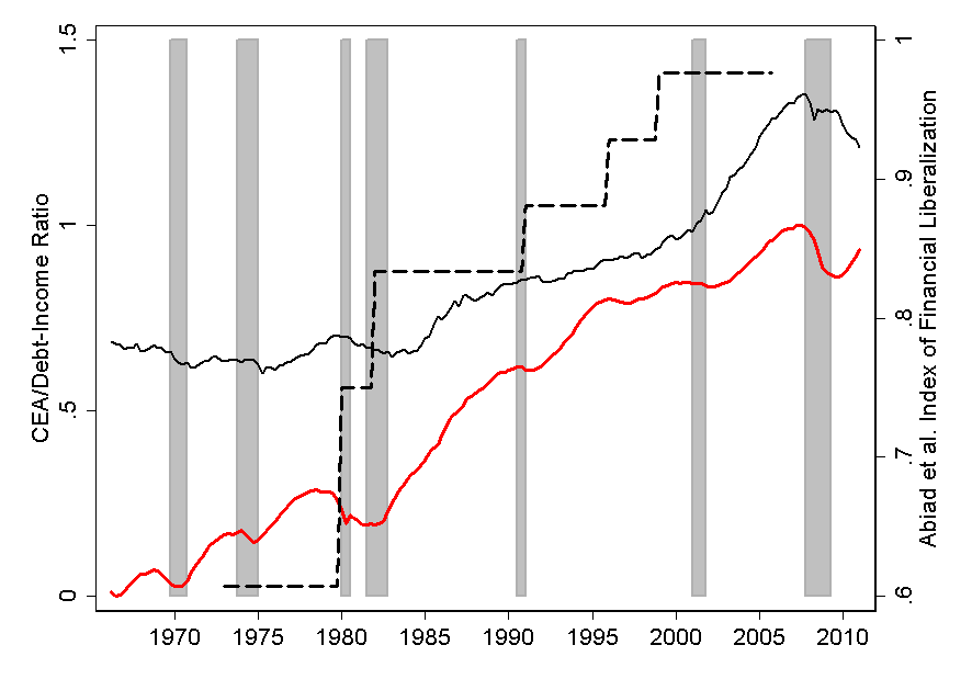
B Comparison of Alternative Measures of Credit Availability
Figure 10 compares three measures of credit availability: our baseline CEA index, the Index of
Financial Liberalization constructed by Abiad, Detragiache, and Tressel (2010) for a number of
countries including the United States, and the ratio of household liabilities to disposable
income.
The Abiad, Detragiache, and Tressel index is a mixture of indicators of financial development:
credit controls and reserve requirements, aggregate credit ceilings, interest rate liberalization,
banking sector entry, capital account transactions, development of securities markets and banking
sector supervision. The correlation coefficient between this measure and CEA is about 90
percent.
For comparison, the figure also includes the ratio of liabilities to disposable income (from the Flow
of Funds), which is however determined influenced by the interaction between credit supply and
demand.
C Reduced Form Regressions with Saving Rate Generated by the Structural Model
Table 4: Reduced-Form Regressions with Saving Rate Estimated by the Structural
Model
| st = γ0 + γmmt + γCEACEAt + γEu 𝔼 tut+4 + γ′Xt + 𝜀t
| | | | Reduced-Form | Additional Variables
|
| | |
| |
|
| Model | Uncertainty | Demographics | Baseline | Time Trend | Gov Sav | Ineq
|
| γ0 | 11.689∗∗∗ | 18.994∗∗∗ | 16.254∗∗∗ | 16.093∗∗∗ | 16.215∗∗∗ | 16.330∗∗∗ |
| | (0.182) | (1.126) | (0.636) | (0.710) | (0.633) | (0.646) |
| γm | | −0.912∗∗∗ | −0.756∗∗∗ | −0.729∗∗∗ | −0.759∗∗∗ | −0.780∗∗∗ |
| | | (0.110) | (0.099) | (0.113) | (0.099) | (0.117) |
| γCEA | | −7.316∗∗∗ | −8.085∗∗∗ | −7.713∗∗∗ | −8.064∗∗∗ | −8.174∗∗∗ |
| | | (0.292) | (0.112) | (0.621) | (0.114) | (0.309) |
| γEu | 0.555∗∗∗ | 0.237∗∗∗ | 0.223∗∗∗ | 0.238∗∗∗ | 0.239∗∗∗ | 0.222∗∗∗ |
| | (0.025) | (0.018) | (0.017) | (0.030) | (0.021) | (0.016) |
| γt | −0.055∗∗∗ | | | −0.002 | | |
| | (0.001) | | | (0.004) | | |
| γold | | −0.191∗∗∗ | | | | |
| | | (0.071) | | | | |
| γgov sav | | | | | 0.014 | |
| | | | | | (0.014) | |
| γinc share | | | | | | 0.010 |
| | | | | | | (0.033) |
| R2 | 0.975 | 0.989 | 0.988 | 0.988 | 0.988 | 0.988 |
| F stat p val | 0.000 | 0.000 | 0.000 | 0.000 | 0.000 | 0.000 |
| DW stat | 1.167 | 2.331 | 2.213 | 2.219 | 2.237 | 2.217 |
| |
Notes: Estimation sample: 1966q2–2011q4. {∗,∗∗,∗∗∗} = Statistical significance at {10,5,1} percent.
Newey–West standard errors, 4 lags.