$©$ September 26, 2022, Christopher D. Carroll OLGModel

The Diamond (1965) OLG Model

This handout and the associated Jupyter notebook, DiamondOLG, present a canonical overlapping generations (OLG) model, like the one originally proposed by Diamond (1965), building on Samuelson (1958).¹

1 Setup

The economy has the following features:

Two generations are alive at any point in time, the young (age 1) and old (age 2).
The size of the young generation in period $t$ is given by $NNN = NNN Ξt t 0$ .
Households work only in the ﬁrst period of life, earning income $Y1,t$ . They earn no income in the second period of life ( $Y2,t+1 = 0$ ).
They consume part of their ﬁrst-period income and save the rest to ﬁnance their consumption when old.
The assets of the young at the end of period $t$ are the source of the capital used for aggregate production in period $t + 1$ , $K = NNN a t+1 t 1,t$ where $a1,t$ is the assets per young household after their consumption in period 1. (For convenience, we assume that there is no depreciation).
The old in period $t$ own the entire capital stock and (because they have no bequest motive) will consume it all, so dissaving by the old in period $t$ will be $NNN a = K t− 1 1,t− 1 t$ . (The old do receive interest on their capital, so their consumption will be $Kt$ plus the interest income $rK t$ , but the $rK t$ component does not aﬀect saving because it is part of both income and consumption).
Labor and capital markets are perfectly competitive and the aggregate production technology is CRS, $Y = F (K, L)$ (recall that this implies that $F(K, L ) = FLL + FK K$ , which is “Euler’s Theorem”.

2 Analysis

Let’s normalize everything by the period- $t$ young population $NNN t$ , writing normalized variables in lower case. Thus the per-young-capita aggregate production function becomes

f(kt) ≡ F (Kt, NNN t)∕NNN t = F (Kt ∕NNN t,1).

(1)

The perfect competition assumption implies that wages and net interest rates are equal to the marginal products of labor and capital, respectively:

W = f(k ) − k f′(k ), t t t t rt = f′(kt).

(2)

To make further progress, we need to make speciﬁc assumptions about the utility function and the aggregate production function. Assume that utility is CRRA, $u (∙) = ∙1− ρ∕(1 − ρ)$ and assume a Cobb-Douglas aggregate production function $𝜀 1− 𝜀 𝜀 F (K, L ) = K L ⇒ f(k ) = k$ .

In this case we can solve for wages and interest rates:

W = (1 − 𝜀)k𝜀 t t rt = 𝜀k 𝜀− 1. t

(3)

The individual’s maximization problem yields the Euler equation:

′ ′ u (c1,t) = βRt+1u (c2,t+1).

(4)

Now let’s assume that utility is logarithmic, $ρ = 1$ , which implies that

=0 ◜-◞◟ -◝ W1,t-+--W2,t+1-∕Rt+1--- c1,t = 1 + β W1,t--- c1,t = 1 + β a1,t = W1,t − c1,t = W1,t (1 − 1∕ (1 + β )) = W1,t (β ∕(1(+ β )) ) β = (1 − 𝜀)k 𝜀t ------- 1 + β =a1,t∕Ξ [ ] ◜◞ ◟◝ (1 − 𝜀)β kt+1 = k 𝜀t ----------- Ξ (1 + β) [ ] dkt+1--= k 𝜀− 1 𝜀-(1-−-𝜀-)β . dkt t Ξ (1 + β )

(5)

The steady-state will be the point where $kt+1 = kt$ . For convenience, deﬁne a constant

𝒬 =

allowing us to rewrite (5) as

𝜀 kt+1 = 𝒬k t.

(6)

Then the steady-state will be the point where $kt+1 = kt = ¯k$

𝜀 ¯k = 𝒬 ¯k 1∕(1− 𝜀) ¯k = 𝒬 .

(7)

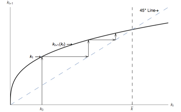
Dynamics of the model can be analyzed using a simple ﬁgure relating the capital stock per capita in period $t + 1$ to that in period $t$ . The solid locus is a graph of equation (5). We depict the 45 degree line because it indicates the set of ‘steady-state’ points where $k = k t+1 t$ and thus any intersection of the 45 degree line with the $kt+1 (kt)$ function indicates a steady-state of the model.

pict

Figure 1:Convergence of OLG Economy to Steady State

The experiment traced out in the ﬁgure is as follows. We start the economy in period $t = 0$ with capital per capita of $k0$ , which, from (5), implies a certain value $k 1$ for capital in period $t + 1 = 1$ . Now think about period $1$ becoming $t$ and period $2$ becoming $t + 1$ . To ﬁnd the correct level of capital implied by the model in period $t + 2$ we need to ﬁnd the point on the 45 degree line that corresponds to $k1$ , then go vertically up from there to ﬁnd $k = k t+1 2$ . When the same set of gyrations is repeated the result is that the level of capital converges to the steady-state level $¯k$ .

3 Social Optimum

We have determined the outcome that will arise in a perfectly competitive economy in which households optimally choose their behavior given market prices with no government intervention.

Often in macroeconomic analysis this constellation of assumptions yields a conclusion that the steady state is optimal (and dynamics are also optimal) according to some plausible criteria. We now examine the optimality properties of the OLG model outcome.

As a preliminary, let’s deﬁne the lifetime utility experienced by the young generation at time $t$ as

v = u(c ) + βu (c ). t 1,t 2,t+1

(8)

Suppose our deﬁnition of optimality reﬂects the choices that would be made by a benevolent social planner who maximizes a social welfare function of the form²

∑∞ Vt = βu (c2,t) + ℶnvt+n n=0

(9)

subject to the economy’s aggregate resource constraint

K◟t--+--F(◝K◜t,-NNN-t)◞ = K◟t+1---+-NNN--tc1◝,◜t-+-NNN--t−-1c2,t◞ Sources Uses

(10)

where the Hebrew letter $ℶ$ reﬂects the social planner’s discount factor and the planner must allocate the society’s resources (“Sources”) between consumption of the two generations alive at time $t$ and the capital stock in period $t + 1$ (“Uses”).

The idea is that the social planner cares about every generation’s lifetime happiness, but discounts the happiness of future generations. (We will discuss why discounting is necessary later in the class).

It is possible to show (using methods not described in this handout; see Blanchard and Fischer (1989) for details) that the socially optimal steady state is characterized by the equation

′ ∗ − 1 1 + f (¯k ) = Ξ ℶ

(11)

In the case of our Cobb-Douglas production function, this becomes

∗ 𝜀− 1 − 1 (¯k ) 𝜀 = Ξ ℶ − 1 ( )1 ∕(𝜀− 1) ∗ Ξℶ − 1 − 1 ¯k = ----------- . 𝜀

(12)

Comparing this to the outcome that will actually arise,

( ) Ξ (1 + β) 1∕(𝜀− 1) ¯k = ----------- , (1 − 𝜀)β

(13)

our point is that there is no particular relationship between the socially optimal outcome and the actual equilibrium outcome that will arise if the social planner is not involved. The actual outcome could have too little capital or too much, and there is no reason to expect it to be the “right” amount.

You might respond by saying that our deﬁnition of optimality here is too strong; we might hope that the economy would at least be able to avoid a Pareto ineﬃcient outcome, even if we can’t expect perfect optimality according to the preferences of some mythical Godlike “social planner.”

It turns out, however, that even Pareto eﬃciency is not guaranteed. (In this context, Pareto eﬃciency must be deﬁned across generations: The economy is Pareto eﬃcient if there is no way to make one generation better oﬀ without making another generation worse oﬀ).

To examine Pareto eﬃciency, start by rewriting the aggregate DBC by dividing by the size of the labor force at time $t$ :

kt + f(kt ) = Ξkt+1 + c1,t + c2,t∕ Ξ

(14)

Deﬁne an index of aggregate per capita consumption as

c = c + c ∕Ξ t 1,t 2,t

(15)

In steady state, $kt+1 = kt = ¯k$ , so if $¯c$ is the steady-state level of $ct$ then the accumulation equation implies

k¯ + f(¯k ) = Ξ ¯k + ¯c f(¯k ) = (Ξ − 1 )¯k + ¯c ◟--◝ ◜--◞ ξ ¯ ¯ f(k) − ξk = ¯c

(16)

Now consider the eﬀects of a change in $¯ k$ on $¯c$ :

( ) d-¯c = f′(¯k) − ξ. d ¯k

(17)

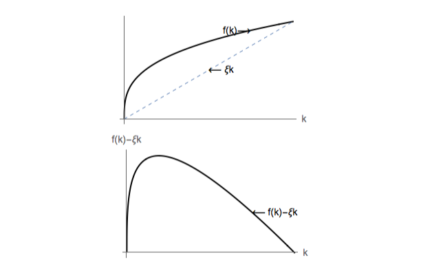
There exists a $¯k$ which maximizes per-capita steady-state consumption:

¯ ¯ max¯ f(k ) − ξ k k

(18)

whose solution is obtained from the FOC

𝜀¯k 𝜀− 1 = ξ ¯k∗∗ = (ξ∕𝜀 )1∕(𝜀− 1),

(19)

and note that this means that for $∗∗ ¯k ≥ ¯k$ an extra bit of capital actually requires a decline in steady-state consumption. An economy in this circumstance of excessive saving is called ‘dynamically ineﬃcient.’

Note further that there is actually a $¯k$ so large that consumption would have to be zero:

¯k 𝜀 = ξk ¯𝜀− 1 k = ξ ¯ 1∕(𝜀− 1) k = ξ .

(20)

These points are illustrated graphically in the remaining ﬁgure.

Figure 2:Gross and Net Per Capita Output as a Function of $k$

pict

References

Blanchard, Olivier, and Stanley Fischer (1989): Lectures on Macroeconomics. MIT Press.

Diamond, Peter A. (1965): “National Debt in a Neoclassical Growth Model,” American Economic Review, 55, 1126–1150, http://www.jstor.org/stable/1809231.

Jefferson, Thomas (1789): “‘The Earth Belongs to the Living’: A Letter to James Madison,” http://infomotions.com/etexts/literature/american/1700-1799/jefferson-letters-256.htm.

Samuelson, Paul A. (1958): “An exact consumption loan model of interest with or without the social contrivance of money,” Journal of Political Economy, 66, 467–482.

Weil, Philippe (2008): “Overlapping Generations: The First Jubilee,” Journal of Economic Perspectives, 22(4), 115–34.