September 13, 2023, Christopher D. Carroll 2PeriodLCModel
September 13, 2023, Christopher D. Carroll 2PeriodLCModel
Irving Fisher (1930) first analyzed the optimization problem of a consumer who faces no uncertainty and lives for two periods.
In its most general form, the household’s lifetime value function can be written

where the first argument reflects consumption in ‘youth’ while the second argument represents consumption in ‘old age’ and we assume that the derivatives with respect to the first and second arguments are positive,
 | (1) |
while the second derivatives are negative,
 | (2) |
The consumer begins the first period with resources of  (think
‘bank balances’) and income of
(think
‘bank balances’) and income of  . Total resources are divided between
consumption and end-of-period assets
. Total resources are divided between
consumption and end-of-period assets  (‘assets after all actions’ in period
 ):
):
 | (3) |
Balances at the beginning of period 2 are equal to end-of-first-period
accumulated assets  , rewarded by a gross interest factor
  :
:
 | (4) |
This is the dynamic budget constraint or DBC for this problem. A DBC links two adjacent periods of time. A more comprehensive kind of constraint is the intertemporal budget constraint (IBC):
 | (5) |
which must be satisfied over an extended (multiperiod) span of time like a lifetime.
For various purposes, it is useful to keep track of human wealth  , defined
as the present discounted value of future labor income (the operator
, defined
as the present discounted value of future labor income (the operator
 denotes the present discounted value of the variable
  from
the perspective of the beginning of period
from
the perspective of the beginning of period  through the end of the
horizon),
through the end of the
horizon),
 | (6) |
Because we have assumed (in (1)) that an additional unit of consumption always yields extra utility, we can reach our first conclusion (as opposed to assumption) in the model: Once the consumer has reached the last period of life, he will consume all available resources:
 | (7) |
This means that the IBC will hold with equality (if it did not, utility could be increased by consuming more in one or both periods). Thus, the IBC can be rewritten as
 | (8) |
The general form that the IBC will take is that the present discounted value of lifetime spending must equal the present discounted value of lifetime resources:
 | (9) |
Substituting in the definition of  means that our problem can now be
stated as:
means that our problem can now be
stated as:
 |
Now we can write the problem as a Lagrange multilier problem, where the maximand is:
 | (10) |
The first order conditions are:
 | (11) |
and substituting the second of these into the first we get
 | (12) |
This is the same condition you get when deciding between two commodities at
a point in time, where we can now think of  as the intertemporal price: How
much of good 2 (consumption in period 2) do I get in exchange for giving up a
unit of good 1 (consumption in period 1).
as the intertemporal price: How
much of good 2 (consumption in period 2) do I get in exchange for giving up a
unit of good 1 (consumption in period 1).
Now suppose that the consumer’s utility is time-separable, and the felicity function (felicity is the utility obtained in a single period of a multi-period problem) is the same in both periods of life, so that
 | (13) |
where  is a time preference factor that specifies how the
consumer trades off utility in period 1 against utility in period
2.1
is a time preference factor that specifies how the
consumer trades off utility in period 1 against utility in period
2.1
From our assumptions (1) and (2) we know that the felicity function must satisfy
 | (14) |
and since the felicity functions are the same in both periods we have that
 | (15) |
Substituting these equations into (12) yields the Euler equation for consumption:
 | (16) |
The Euler equation is a central result in intertemporal optimization theory, and will be used again and again as the course progresses. It is therefore worth studying carefully to be sure you understand it thoroughly.
To help obtain the intuition for why the Euler equation is necessary for
optimality, consider the following thought experiment. Designate  and
and  as
the optimal levels of consumption in this problem, the levels that solve the
maximization problem under some set of circumstances. Thus, the highest
attainable utility is
as
the optimal levels of consumption in this problem, the levels that solve the
maximization problem under some set of circumstances. Thus, the highest
attainable utility is
 | (17) |
Now consider reducing consumption by some small amount  in period 1,
investing that
in period 1,
investing that  so that it grows to
  in period 2, and then consuming it in
period 2. What happens to utility?
in period 2, and then consuming it in
period 2. What happens to utility?
Taking first-order Taylor expansions, the levels of first-period and second-period utility are now
 | (18) |
Now the difference between the maximum possible utility and the new situation is given by
![u(c ∗)+ βu (c∗)− [u (c∗) − u ′(c ∗)𝜖 + β (u (c∗) + u ′(c ∗)R 𝜖)] = u′(c∗)𝜖− βu ′(c ∗)R𝜖.
1 2 1 1 2 2 1 2](2PeriodLCModel39x.svg) | (19) |
But it must be the case that (19) is approximately equal to zero. To see why,
suppose it were a negative number. That would mean that moving from the
original situation with  to the new situation with
 resulted in an increase in utility. But we assumed
that
resulted in an increase in utility. But we assumed
that  were already the utility-maximizing choices, which clearly could not
be true if adjusting
were already the utility-maximizing choices, which clearly could not
be true if adjusting  downward by
  and
and  upward by
  increased
utility. Similarly, if the expression were positive, then utility could be increased
by doing the opposite (i.e. increasing consumption in period 1 by
increased
utility. Similarly, if the expression were positive, then utility could be increased
by doing the opposite (i.e. increasing consumption in period 1 by  and
reducing it in period 2 by
and
reducing it in period 2 by  ). Thus, in either case if the expression is not zero,
we have a contradiction to the assumption that
). Thus, in either case if the expression is not zero,
we have a contradiction to the assumption that  and
and  are the
utility-maximizing choices.
are the
utility-maximizing choices.
To make further progress, it is necessary to make more specific assumptions about the structure of the utility function. The most common assumption is that utility takes the Constant Relative Risk Aversion form,
 | (20) |
with marginal utility
 | (21) |
Consider equation (16) with CRRA utility,
 | (22) |
Now note that this equation allows us to calculate the intertemporal elasticity
of substitution as the change in the ratio of the log of  to the log change in
the intertemporal price
to the log change in
the intertemporal price  :
:
 | (23) |
Next note that from (22) we can calculate the PDV of lifetime consumption from the perspective of the first period of life as
 | (24) |
Now we can use the intertemporal budget constraint:
 | (25) |
Thus, we have solved the two-period life cycle saving problem for the
consumption function  relating the level of consumption to all of the
parameters of the problem.
relating the level of consumption to all of the
parameters of the problem.
One of the surprising features of the solution goes by the name of “Fisherian
Separation”: Notice that the profile of consumption growth over the lifetime is
given by (22) regardless of the shape of the income profile. For two consumers
with the same total amount of lifetime wealth (combined  and
and  , the level
and growth rates of consumption over the lifetime will be identical whether the
consumer’s lifetime wealth is entirely concentrated in the first period (that
is,
, the level
and growth rates of consumption over the lifetime will be identical whether the
consumer’s lifetime wealth is entirely concentrated in the first period (that
is,  ), entirely concentrated in the last period (
 ), split
half-and-half, or organized any other way. Fisherian Separation is a pervasive
feature of models that combine perfect foresight and a lack of liquidity
constraints.
), split
half-and-half, or organized any other way. Fisherian Separation is a pervasive
feature of models that combine perfect foresight and a lack of liquidity
constraints.
A common assumption (for simplicity, not realism) is that
 , which is equivalent to assuming that the utility function is
logarithmic:2
, which is equivalent to assuming that the utility function is
logarithmic:2
 | (26) |
In this case it turns out that we can simply substitute  into the solution
for consumption, obtaining
into the solution
for consumption, obtaining
 | (27) |
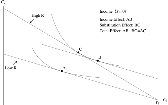
The classic graphical analysis of this problem is shown in figure 1.
The top figure depicts a situation in which all of the consumer’s lifetime
income is earned in the first period of life. The budget constraint in the initial
situation, associated with a “Low  ”, yields an optimal consumption choice
labeled as point
”, yields an optimal consumption choice
labeled as point  where the budget constraint is tangent to the indifference
curve. When the interest factor is increased to the “High
where the budget constraint is tangent to the indifference
curve. When the interest factor is increased to the “High  ” situation, the
optimal consumption choice moves to point
” situation, the
optimal consumption choice moves to point  .
.
Note first that if all income is earned in the first period of life, an increase in the interest factor is unambiguously good for the consumer - the set of consumption possibilities is strictly larger.
Second, the movement from point  to point
  can be decomposed into
two parts: an income effect
can be decomposed into
two parts: an income effect  and a substitution effect
  .
.
Call the low and the high interest factors respectively  and
and  .
.
The income effect is the answer to the question “Suppose we wanted to change
lifetime value by the same amount as it is changed by going from  to
to  , but
we wanted to achieve this change in value at the initial interest factor
, but
we wanted to achieve this change in value at the initial interest factor
 . Supposing we gave the consumer enough extra initial resources to
achieve the change in value, how would their consumption allocation
change?”
. Supposing we gave the consumer enough extra initial resources to
achieve the change in value, how would their consumption allocation
change?”
In order to relate this back to the algebraic analysis above, it will be useful
to rewrite lifetime value as a function simply of initial resources and
the interest factor (taking  and other parts of the problem as
given):
and other parts of the problem as
given):
 | (28) |
Using this function, the income effect is obtained as the value of  in the
equation
in the
equation  .
.
The substitution effect is the answer to the question, “Staying on the new
indifference curve, how much does the allocation of consumption change as a
consequence of the difference in interest factors between  and
and  ?” This is
captured in the movement from
?” This is
captured in the movement from  to
to  .
.
Note that the income and the substitution effects on  are opposite in sign.
A higher interest factor gives consumers the incentive to substitute future for
current consumption (
are opposite in sign.
A higher interest factor gives consumers the incentive to substitute future for
current consumption ( is lower at point
  than at
  ). But a higher
interest factor also gives consumers the ability to consume more in both periods.
Whether
). But a higher
interest factor also gives consumers the ability to consume more in both periods.
Whether  rises or falls in response to the increase in interest factors
will depend on the relative magnitudes of the income and substitution
effects.
rises or falls in response to the increase in interest factors
will depend on the relative magnitudes of the income and substitution
effects.
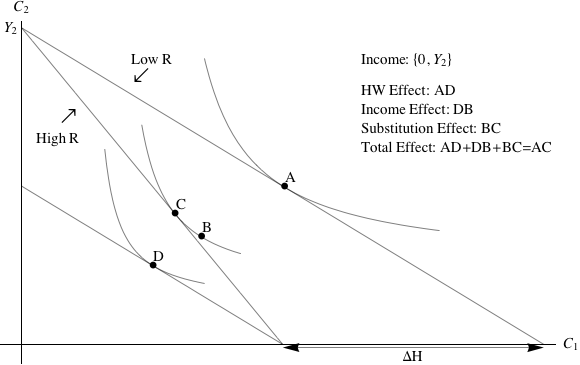
The lower figure shows a similar experiment, with the sole difference that the consumer’s lifetime resources are exclusively concentrated in period 2.
In this case, the period 1 consumer must borrow against future income in order to consume anything. An increase in interest factors is therefore unambiguously bad (the available set of consumption choices is strictly smaller).
The optimal choice again moves from point  to point
  . However, we now
decompose the movement into three parts. The first part is called the human
wealth effect. It captures the fact that the present discounted value of lifetime
resources
. However, we now
decompose the movement into three parts. The first part is called the human
wealth effect. It captures the fact that the present discounted value of lifetime
resources  is smaller when interest rates are higher; the magnitude of the
change in human wealth is depicted on the horizontal axis of the figure. The
human wealth effect is the consequence that an equivalent change in lifetime
resources would have in the absence of any change in interest factors. So
the human wealth effect takes the consumer from point
is smaller when interest rates are higher; the magnitude of the
change in human wealth is depicted on the horizontal axis of the figure. The
human wealth effect is the consequence that an equivalent change in lifetime
resources would have in the absence of any change in interest factors. So
the human wealth effect takes the consumer from point  to point
 .
.
Notice that once we have computed the human wealth effect, if we treat point
 as the starting point of our analysis, the remaining analysis is identical to
that for the upper figure: We can increase the interest factor from
as the starting point of our analysis, the remaining analysis is identical to
that for the upper figure: We can increase the interest factor from  to
to  ,
which causes the equilibrium point to change from point
,
which causes the equilibrium point to change from point  to point
  , a
movement that can be decomposed into an income effect
, a
movement that can be decomposed into an income effect  (analogous to the
income effect
(analogous to the
income effect  in the original analysis) and a substitution effect
 .
.
The terminology here is a modification (refinement) of the terminology often employed in micro textbooks, where the “income effect” is defined in a way that would incorporate both what I am calling the income effect and what I am calling the human wealth effect.
The reason to make this distinction is that it is important to distinguish between effects on behavior caused by the fact that the discounted value of future income is changed, and effects caused by the fact that the income that will be earned on savings is different. Summers (1981) vigorously made the point that in standard life cycle models, the quantitative magnitude of the human wealth effect dwarfs the size of either the income or the substitution effects, because for most people most of their lifetime income is in the future.
Fisher, Irving (1930): The Theory of Interest. MacMillan, New York.
Frederick, Shane, George Loewenstein, and Ted O’Donogue (2002): “Time Discounting and Time Preference: A Critical Review,” Journal of Economic Literature, XL(2), 351–401.
Samuelson, Paul A (1937): “A note on measurement of utility,” The Review of Economic Studies, 4(2), 155–161.
Samuelson, Paul A. (1958): “An Exact Consumption-Loan Model of Interest with or without the Social Contrivance of Money,” Journal of Political Economy, 66(6), 467–482.
Summers, Lawrence H. (1981): “Capital Taxation and Accumulation in a Life Cycle Growth Model,” American Economic Review, 71(4), 533–544, http://www.jstor.org/stable/1806179.