
ctDiscrete CDC response to PT edits for EJ resubmission
_____________________________________________________________________________________
Abstract
We present an analytically tractable model of the effects of nonfinancial risk on intertemporal choice. Our
framework can be adopted in contexts where modelers have until now chosen not to incorporate serious
nonfinancial risk because the available methods did not yield transparent insights. Our model produces an
intuitive formula for target assets, and we show how to analyze transition dynamics using a familiar
Ramsey-style phase diagram. Despite its starkness, the model captures many of the key implications of
nonfinancial risk for intertemporal choice.
risk, uncertainty, precautionary saving, buffer stock saving
C61, D11, E24
| PDF: | http://econ.jhu.edu/people/ccarroll/papers/ctDiscrete.pdf |
| Web: | http://econ.jhu.edu/people/ccarroll/papers/ctDiscrete/ |
| Archive: | http://econ.jhu.edu/people/ccarroll/papers/ctDiscrete.zip |
| (Contains Mathematica and Matlab code solving the model) |
1Carroll: ccarroll@jhu.edu, Department of Economics, Johns Hopkins University, Baltimore Maryland 21218, USA; and National Bureau of Economic Research. http://econ.jhu.edu/people/ccarroll 2Toche: contact@patricktoche.com, Christ Church, Oxford OX1 1DP, UK.
The Merton-Samuelson model of portfolio choice is the foundation for the vast literature analyzing financial risk,2 not because it offers conclusions that cannot be obtained from other frameworks,3 but because it is easy to use and its key insights emerge in a way that is natural, transparent, and intuitive — in a word, the Merton-Samuelson model is tractable.
Unfortunately, nonfinancial risk4 (which is much more important than financial risk for most households)5 has proven more difficult to analyze. Of course, a large and impressive numerical literature has carefully computed the effects of specific nonfinancial risks in a variety of particular contexts.6 But because the computational methods necessary to solve such models are daunting and the insights that emerge are not easy to explain, much of the economic literature (and much graduate-level instruction) has dodged the question of how nonfinancial risk influences choices, by assuming perfect insurance markets or perfect foresight or risk neutrality or quadratic utility or Constant Absolute Risk Aversion, or by attempting only to match aggregate risks (which are orders of magnitude smaller than idiosyncratic risks). These approaches rob the question of its essence, either by assuming (counterfactually) that markets transform nonfinancial risk into financial risk or by making implausible assumptions crafted to generate the implausible conclusion that decisions are largely or entirely unaffected by nonfinancial risk.7
Our contribution is to offer a tractable model that captures the main features of realistic models of the optimal response to nonfinancial risk, but without the customary technical difficulties. The model is a natural extension of the no-risk perfect foresight framework. Its solution is characterized by simple, intuitive equations and we show how the model’s results can be analyzed using a phase diagram like that of the canonical Ramsey growth model.
The trick that yields tractability is to distill all nonreturn risk into a stark and simple possibility: A one-time uninsurable permanent loss in nonfinancial income. Our view is that the consumer’s response to this single, tractable risk captures most of the substantive essence of the results obtained by the numerical literature under more realistic but more complex assumptions about income dynamics. Indeed, our view is that our model matches essentially all of the qualitative and even some of the quantitative implications of such models.
The kind of real-world shock that our μ shock most closely resembles is permanent disability from which no recovery is possible. We take the liberty of interpreting the shock more loosely, as capturing the role of unemployment or forced retirement risk, for several reasons. Most importantly, compared to perfect foresight models, the key qualitative characteristic that distinguishes models with a meaningful precautionary motive is the concavity of the consumption function (see Carroll and Kimball (1996) for general proof that uncertainty induces consumption concavity), which our model generates in the simplest way we know of. While exact quantitative details of the consumption function generated by models with more realistic formulations of income dynamics will differ from those we obtain, our purpose here is more qualitative and analytical than quantitative and empirical.8
The same framework could be interpreted to apply in other contexts as well; for instance, the risk faced by a country whose exports are dominated by a commodity whose price might collapse permanently (e.g., oil exporters, if cold fusion had worked).9
The optimal response to any such risk is to aim to accumulate a buffer stock of precautionary assets. The existing literature has computed the numerical value of the target under specific parametric assumptions, but has struggled to present an intuitive picture of the determinants of that target. Here, we are able to derive an analytical formula for the target level of wealth, and show how the precautionary motive (nonlinearly) interacts with the other saving motives that have been well understood since Irving Fisher (1930)’s work: The income, substitution, and human wealth effects.
Thanks to the model’s tractability, we are able to derive a simple expression that shows how the familiar perfect-foresight consumption Euler equation is modified by the presence of our risk. The effect of our risk on consumption growth is related to the probability of the risky event, to its magnitude, to the consumer’s degree of risk aversion, to the consumer’s wealth, and to all of the parameters of the model (including risk aversion and time preference). We obtain an exact analytical expression (not a log-linearized one) for the combined value of the higher-order Euler equation terms at the target.
With this expression in hand, the intuition for why empirical Euler equation estimation is problematic comes into clear focus, and the problems that have bedeviled the Euler equation literature can be plainly articulated and understood (see section 2.2.11).
A tractable model like ours can be used as a reference point for more specialized models, complementing the perfect foresight, certainty equivalent, or perfect markets models that are currently so widely used because of their tractability. Even computation-intensive literatures like heterogeneous-agents macroeconomics may find ours a useful ‘toy model’ with which to exposit some of the subtle points that numerical simulations deliver without interpretation.10
If the consequences of nonfinancial risk were numerically trivial, a tractable model would be of little interest. But the success of the growing heterogeneous-agents literature in macroeconomics suggests that the profession is increasingly coming to the view that something essential is missed when idiosyncratic risk is ruled out.
Part, at least, of what is missing in such models is the ability to analyze the consequences of wealth heterogeneity. In the absence of nonfinancial risk, Uzawa (1968) pointed out that if infinite-horizon agents have heterogeneous preferences, the most patient agent ends up owning all aggregate wealth in equilibrium (a point that was anticipated, but not fully developed, in Ramsey (1928) and is fleshed out in Becker and Foias (1987)). Mathematically, this is because any agent who is impatient (at the prevailing interest rate) will choose to run down his wealth to its minimum possible value, while any agent who is patient relative to that interest rate will choose to accumulate indefinitely.
If we grant that there is even a small amount of heterogeneity in time preference rates, relative risk aversion, expected income growth, mortality risk, age, or any other factor that influences intertemporal choice, a model without nonfinancial risk leads to radical wealth inequality that is even greater than the substantial but not unlimited differences in wealth in the cross-sectional data.
In such a world, the representative agent model’s approximation of behavior around the aggregate steady-state wealth-to-income ratio is an approximation around a wealth-to-income ratio that is arbitrarily far from the wealth-to-income ratio that anyone in the economy will actually experience. To take a simple example, suppose everybody has the same nonfinancial income, borrowing is ruled out, and suppose that 5 percent of agents are “patient” and 95 percent are “impatient.” Then the patient agents will have a wealth-to-income ratio equal to about 20 times the aggregate ratio, while impatient agents will have a wealth-to-income ratio of zero. Since no approximation is good at vast distances from the approximating point, there is no reason to suppose that approximating behavior around the aggregate wealth-to-income ratio will provide even a remotely accurate description of the behavior of the actual aggregate economy with heterogeneous agents but perfect foresight. Indeed, the logic of the model is that essentially nobody will hold a level of wealth close to the representative agent’s level of wealth, around which everybody’s behavior is approximated.
The appeal of introducing nonfinancial risk is that the precautionary motive prevents wealth from asymptoting to its lower bound for households who are impatient relative to the interest rate. Each kind of household’s behavior can be approximated around a target level of wealth that reflects their actual wealth, rather than around the representative agent’s wealth. In the presence of heterogeneity and nonfinancial risk, the only agents whose behavior is not captured by the model are those who are patient relative to the equilibrium interest rate. Since the wealth of those agents is heading to infinity, their behavior may be reasonably approximated by the behavior of a perfect foresight agent.
For concreteness, we analyze the problem of an individual consumer facing a labor income risk. Other interpretations (like those mentioned in the introduction) are left for future work or other authors.11
The aggregate wage rate, Wt, grows by a constant factor G from the current time period to the next, reflecting exogenous productivity growth:
The interest rate is exogenous and constant (the economy is small and open); the interest factor is denoted R.12 Define m as market resources (financial wealth plus current income), a as end-of-period assets after all actions have been accomplished (specifically, after the consumption decision), and b as bank balances before receipt of labor income. Individuals are subject to a dynamic budget constraint (DBC) that can be decomposed into the following elements:
where ℓ measures the consumer’s labor productivity (hours of work for an employed consumer are assumed to be exogenous and fixed) and ξ is a dummy variable indicating the consumer’s employment state: Everyone in this economy is either employed (ξ = 1, a state indicated by the letter ‘e’) or unemployed (ξ = 0, a state indicated by ‘u’). Thus, labor income is zero for unemployed consumers.13There is no way out of unemployment; if an individual becomes unemployed, that individual remains
unemployed forever, ξt = 0 ξt+1 = 0 ∀ t.
Consumers have a CRRA utility function u(c) = c1−ρ∕(1 −ρ), with ρ > 1, and they discount future utility geometrically by β per period. We show below that the simplicity of the unemployed consumer’s behavior is what makes employed consumer’s problem tractable. The solution to the unemployed consumer’s optimization problem is simply:14
where κu is the ‘marginal propensity to consume’ out of total wealth (MPC), which for the unemployed consists in bank balances b only, because we have assumed that noncapital income of the unemployed is zero. This is for simplicity only; incorporation of an unemployment insurance system that pays a fixed proportion of the final employed wage is straightforward, because in the absence of further uncertainty the value of those future payments is equivalent to receipt of a lump sum equal to the present discounted value of the payments. The accompanying solution code for the model, in fact, incorporates a parameter measuring the generosity of the unemployment insurance system, and the solutions presented in the paper are those produced when that parameter is set to zero.Table 6 summarizes our notation. We follow the terminology in Carroll (2016b), where a detailed discussion of the concepts is provided. We impose a condition on parameters to ensure that the marginal propensity to consume out of total wealth is positive, κu > 0:
The unemployed consumer will be spending enough to make the ratio of financial wealth to human wealth decline over time. The interpretation is that the consumer must not be so patient that a boost to wealth would fail to boost current consumption. An alternative (equally correct) interpretation is that the condition guarantees that the present discounted value (PDV) of consumption for the unemployed consumer remains finite.15Note that our results do not depend on the stronger16 restriction that is often imposed:
Here the consumer will choose to spend more than the amount that would permit constant consumption; such a consumer’s absolute level of wealth declines over time, together with consumption, since consumption and wealth are proportional. Carroll (2016b) calls the first type of consumer “return impatient” and the second, more impatient type “absolutely impatient.” The restriction we impose, therefore, is the Return Impatience Condition (RIC) defined in Carroll (2016a).The consumer’s preferences are the same in the employment and unemployment states; only exposure to risk differs. There are two effects at work. On the one hand, the precautionary saving motive is inversely related to wealth, so that ‘poor’ consumers choose to save more than ‘rich’ consumers. On the other hand, the impatience motive is independent of wealth. The two effects thus influence wealth in opposite directions. Under our parameter restrictions, there is a point at which prudence and impatience are in exact balance. This balance condition defines the target wealth-to-income ratio.
A consumer who is employed in the current period has ξt = 1; if this person is still employed next period (ξt+1 = 1), market resources will be:
 | (9) |
However, there is no guarantee that the consumer will remain employed: Employed consumers face a constant risk μ of becoming unemployed.
We assume that ℓ grows by a factor (1 −μ)−1 every period,
 | (10) |
because under this assumption, for a consumer who remains employed, labor income will grow by factor Γ = G∕(1 −μ), so that the expected labor income growth factor for employed consumers is the same G as in the no-risk perfect foresight case:
![𝔼t[Wt +1ℓt+1ξt+1] = Γ Wt ℓt (μ × 0 + (1 − μ) × 1)
𝔼t[Wt+1ℓt+1ξt+1]
⇒ Wt ℓt = Γ (1 − μ) = G = no -risk growth](ctDiscrete12x.svg)
The usual steps lead to the standard consumption Euler equation. Using i ∈ {e,u} to stand for the two possible states,
![′ e [ ′ i ]
u(ct) = R β𝔼t u (ct+1)
⌊|(ci )−ρ⌋|
⇒ 1 = R β𝔼t|||⌈ -t+e1 |||⌉. (11)
ct](ctDiscrete13x.svg)
Henceforth nonbold variables will be used to represent the bold equivalent divided by the level of permanent labor income for an employed consumer, e.g. ce t = ce t∕(Wtℓt); thus we can rewrite the consumption Euler equation as:
where the term in braces is a probability-weighted average of the growth rates of marginal utility in the case where the consumer remains employed (the first term) and the case where the consumer becomes unemployed (the second term).
An intuitive interpretation of the consumption Euler equation is readily available. Re-write equation (12) in terms of the growth rate of consumption in the employment state:
where is the factor by which the level of consumption c would grow in a perfect foresight no-risk model. To understand (13), it is useful to consider an approximation. Define ∇t+1 ≡  , the proportion by
which the consumption ratio next period would be lower in the event of a transition into unemployment;
we refer to this loosely as the size of the ‘consumption risk.’ Define ω, the ‘excess prudence’ factor, as
ω = (ρ−1)∕2.17
Applying a Taylor approximation to (13) (see appendix A.1) yields:
, the proportion by
which the consumption ratio next period would be lower in the event of a transition into unemployment;
we refer to this loosely as the size of the ‘consumption risk.’ Define ω, the ‘excess prudence’ factor, as
ω = (ρ−1)∕2.17
Applying a Taylor approximation to (13) (see appendix A.1) yields:
The approximations in (15) or (16) capture the essence of equation (13). As a consequence of missing insurance markets, consumption growth depends on the employment outcome; the consumption ratio if employed next period ce t+1 is greater than if unemployed cu t+1, so that ∇t+1 is positive. In the limit case, if we let the transition probability μ go to zero, consumption risk ∇ vanishes and thus ce t+1∕ce t approaches its perfect-foresight value Þ. Equation (15) thus shows that the presence of unemployment risk boosts consumption growth by an amount proportional to the probability of becoming unemployed μ multiplied by a factor that is increasing in the amount of consumption risk ∇. Equation (16) shows that, in the logarithmic case, the precautionary boost to consumption growth is directly proportional to the size of the consumption risk.
The effect of risk on saving is transparent. For a given value of me t, risk has no effect (by construction) on the PDV of future labor income and human wealth, but the larger is μ, the faster consumption growth must be, as equation (15) shows. For consumption growth to be faster while keeping its PDV constant, the level of current ce must be lower. Thus, the introduction of a risk of unemployment μ induces a (precautionary) increase in saving.
In the (persuasive) case where ρ > 1, equation (15) implies that a consumer with a higher degree of prudence (larger ρ and therefore larger ω) will anticipate greater consumption growth. This reflects the greater precautionary saving motive induced by a higher degree of prudence.
To compute the steady state of the model, we explicitly solve for the Δce t+1 = 0 and Δme t+1 = 0 loci.
Consider a consumer who is employed in period t and at his steady-state target value of be t. Substituting ce t+1 = ce t = ce and cu t+1 = cu into (13) and rearranging yields the ratio of consumption in the two states at the buffer-stock target value:
Next, the dynamic budget constraint (4) may be used to express cu in terms of ce. If a transition into unemployment occurs at date t, then mt+1u = b t+1u = b t+1e, implying: where the consumption function (5) ct+1u = κum t+1u was used. Then, equations (17) and (18) may be solved for ce in terms of me; straightforward algebra shows that the Δce t+1 = 0 locus is characterized by proportionality between ce and me: where To characterize the Δme t+1 = 0 locus, we normalize the budget constraint (4) for the employment state, paralleling the normalization for the unemployment state detailed in (18), The target values me and ce solve the linear system formed by equations (19) and (21). Equation (19) is a steady-state version of the Euler equation of the employed worker, conditional upon remaining employed, where the marginal utility in the unemployment state is expressed in terms of wealth. Note that while the steady-state condition is associated with a (hypothetical) steady state in which unemployment is never actually realized, the aversion to the risk of unemployment exerts an effect on that steady state. Equation (21) is a steady-state version of the budget constaint of the employed worker. To each steady-state condition is associated a locus used to depict the phase diagram of the system in Figure 1. The buffer-stock target ratio is given by the intersection of the two loci. Since the conditions are linear, the intersection is unique (our parameter restrictions ensure existence).The appendix details the complete solution. Before we turn to an analysis of the target level of me, we briefly discuss parameter restrictions needed to ensure its existence.
In section 2.1.2, we derived a set of parameter restrictions from the problem of the unemployed consumer that ensure κu > 0 (the RIC). In this section, we derive a further set of restrictions from the problem of the employed consumer. The solution in employment is characterized by me t > ce t > 0 because, with CRRA preferences, zero consumption carries an infinite penalty, implying that a consumer facing the risk of perpetual unemployment will never borrow. Therefore, as may be seen from equation (17), steady-state consumption is positive only if:
In the limit, as μ approaches zero, the condition reduces to Þ∕Γ < 1, or equivalently: It is useful to compare condition (23) with condition (7). The condition ensures that such a consumer facing no risk (μ = 0) would be sufficiently impatient to choose a wealth-to-permanent-income ratio that would be falling over time. The restriction we impose, therefore, is a weak form of the Growth Impatience Condition (GIC) defined in Carroll (2016b).18The target level of the ratio of wealth to income me may be written in closed form:
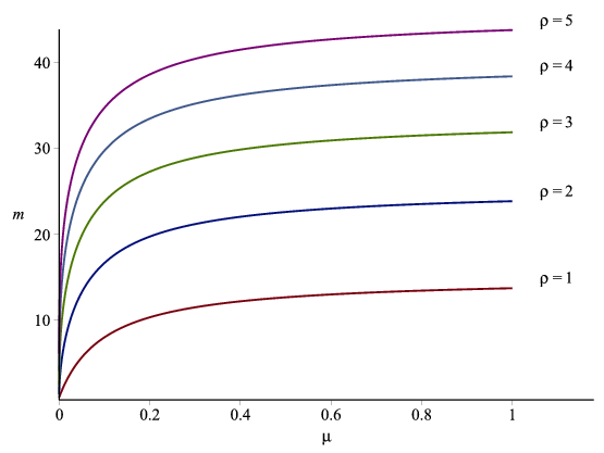
where we have used the shorthand Þ ≡ (Rβ)1∕ρ.We now illustrate the analytics of the target formula with two special cases.
The first special case we consider is ρ = 1 (logarithmic utility). The appendix shows that an approximation of the target formula reduces to:
where19 γ ≡ Γ −1, r ≡ R −1, 𝜗 ≡ (1∕β) −1. This expression encapsulates several of the key intuitions of the model. The human wealth effect of labor income growth (conditional upon remaining employed) is captured by the first γ term in the denominator; for any calibration for which the denominator is positive, increasing γ reduces the target level of wealth. This reflects the fact that a consumer who anticipates being richer in the future will choose to save less in the present, and the result of lower saving is smaller wealth. The human wealth effect of interest rates is correspondingly captured by the −r term, which goes in the opposite direction to the effect of income growth, because an increase in the rate at which future labor income is discounted constitutes a reduction in human wealth. An increase in the rate at which future utility is discounted, 𝜗, reduces the target wealth level. Finally, a reduction in unemployment risk raises (γ + 𝜗 −r)∕μ and therefore reduces the target wealth level.20 ,21Note that the different effects interact with each other, in the sense that the strength of, say, the human wealth effect of interest rates will vary depending on the values of the other parameters.
The assumption of log utility is implausible; empirical estimates from structural estimation exercises (e.g. Gourinchas and Parker (2002), Cagetti (2003), or the subsequent literature) typically find estimates considerably in excess of ρ = 1, and evidence from Barsky, Juster, Kimball, and Shapiro (1997) suggests that values of 5 or higher are not implausible. The next case illuminates how risk aversion affects the target formula for ρ > 1.
The second special case we consider is 𝜗 = r. The appendix shows that an approximation of the target formula reduces to:
Compare the target level in (26) with (25). The key difference is that (26) contains an extra term involving ω, which measures the amount by which relative risk aversion exceeds the logarithmic benchmark. An increase in ω reduces the denominator of (26) and thereby raises the target level of wealth, just as would be expected from an increase in the intensity of the precautionary motive.In the ω > 0 case, the interaction effects between parameter values are particularly intense for the (γ∕μ)2 term that multiplies ω; this implies, e.g., that a given increase in unemployment risk can have a greater effect on the target level of wealth for a consumer who is more prudent.
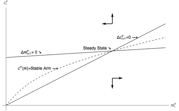
Figure 1 presents the phase diagram of system (19)-(21) under our baseline parameter values. Since the employed consumer never borrows, market resources never fall below the value of current labor income, which is the value selected for the origin of the diagram.22 An intuitive interpretation is that the Δme = 0 locus characterized by (21) shows how much consumption ce t would be required to leave resources me t unchanged so that me = me t.23 Thus, any point below the Δme = 0 line would have consumption below the break-even amount, implying that wealth would rise. Conversely for points above Δme = 0. This is the logic behind the horizontal arrows of motion in the diagram: Above Δme = 0 the arrows point leftward, below Δme = 0 the arrows point rightward.
The intuitive interpretation of the Δce = 0 locus characterized by (19) is more subtle.
Note first that expected consumption growth depends on the amount by which consumption would fall if the unemployment state were realized, an amount which depends on the ce∕cu ratio. For any level of resources, the further below the break-even level actual consumption is, the smaller the ce∕cu ratio is, and therefore the smaller consumption growth is. Thus, points below the Δce = 0 locus are associated with negative values of Δce (and points above it are associated with positive values). This is the logic behind the vertical arrows of motion in the diagram: Above the Δce = 0 locus the arrows point upward; below the Δce = 0 locus the arrows point downward.
The slope of the locus depends essentially on the degree of impatience, as can be seen most directly by considering (20). As μ approaches zero, the proportionality between ce and me approaches π = 1; this is because the vanishing risk of unemployment makes borrowing against future income more and more tempting, and (given our assumption of impatience), the target level of wealth will approach closer and closer to its minimum feasible value on the 45 degree line. On the other hand, as μ approaches 1 (so that receiving future income becomes more and more unlikely) the temptation exerted by that future income diminishes, so the pressure of impatience is smaller and the target level of wealth is greater. While the interactions between the terms in (20) are nonlinear, a similar story can be told for the other indicators of impatience: Greater impatience tilts the slope of the curve upward, and vice versa.
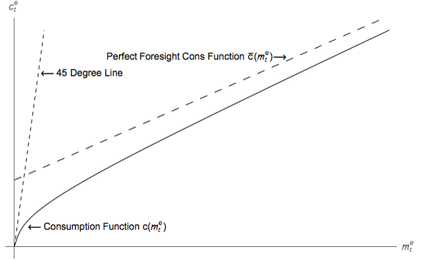
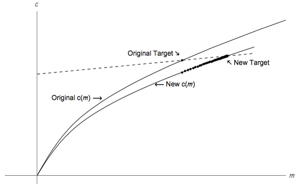
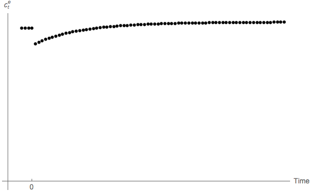
Figure 2 shows the optimal consumption function c(m) for an employed consumer (dropping the e superscript to reduce clutter). This is of course the stable arm of the phase diagram. Also plotted are the 45 degree line along which ct = mt and
where
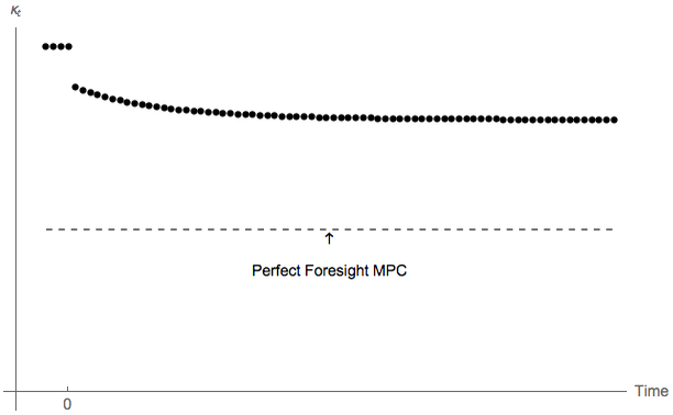
The consumption function c(m) is concave: The marginal propensity to consume  (m) ≡ dc(m)∕dm
is higher at low levels of m because the intensity of the precautionary motive increases as resources m
decline.26
The MPC is higher at lower levels of m because the relaxation in the intensity of the precautionary
motive induced by a small increase in m (Kimball, 1990) is relatively larger for a consumer
who starts with less than for a consumer who starts with more resources (Carroll and
Kimball, 1996).
(m) ≡ dc(m)∕dm
is higher at low levels of m because the intensity of the precautionary motive increases as resources m
decline.26
The MPC is higher at lower levels of m because the relaxation in the intensity of the precautionary
motive induced by a small increase in m (Kimball, 1990) is relatively larger for a consumer
who starts with less than for a consumer who starts with more resources (Carroll and
Kimball, 1996).
To see this important point, consider a counterfactual. Suppose the consumer were to spend all his resources in period t, i.e. ct = mt. In this situation, if the consumer were to become unemployed in the next period, he would then be left with resources mu t+1 = (mt −ct)R∕Γ = 0 , which would induce consumption cu t+1 = κumu t+1 = 0, yielding negative infinite utility. A rational, optimizing consumer will always avoid such an eventuality, no matter how small its likelihood may be. Thus the consumer never spends all available resources.27 This implication is illustrated in figure 2 by the fact that consumption function always remains below the 45 degree line.
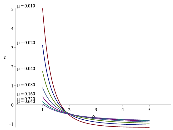
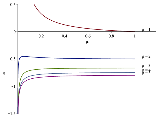
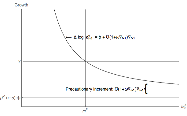
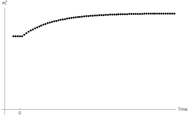
Figure 3 illustrates some of the key points in a different way. It depicts the growth rate of consumption ce t+1∕ce t as a function of me t. Consumption growth is equal to what it would be in the absence of risk, plus a precautionary term; for algebraic verification, multiply both sides of (13) by Γ to obtain:
Observe that the contribution of the precautionary motive becomes arbitrarily large as mt → 0, because cu t+1 = κumu t+1 = (mt −c(mt))κuR∕Γ approaches zero as m t → 0; that is, as resources me t decline, expected consumption growth approaches infinity. The point where consumption growth is equal to income growth is at the target value of me.We are finally in position to get an intuitive understanding of how the model works and why a target wealth ratio exists. On the one hand, consumers are growth-impatient: It cannot be optimal for them to let wealth become arbitrarily large in relation to income. On the other hand, the precautionary motive intensifies as the level of wealth falls. The two effects work in opposite directions. As resources fall, the precautionary motive becomes stronger, eventually offsetting the impatience motive. The point at which prudence becomes exactly large enough to match impatience defines the target wealth-to-income ratio.
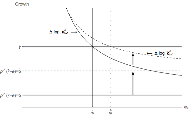
It is instructive to work through a couple of comparative dynamics exercises. In doing so, we assume that all changes to the parameters are exogenous, unexpected, and permanent. Figure 4 depicts the effects of increasing the interest rate to r > r. The no-risk consumption growth locus shifts up to the higher value þr ≈ ρ−1(r −𝜗), inducing a corresponding increase in the expected consumption growth locus. Since the expected growth rate of labor income remains unchanged, the new target level of resources me is higher. Thus, an increase in the interest rate raises the target level of wealth, an intuitive result that carries over to more elaborate models of buffer-stock saving with more realistic assumptions about the income process (Carroll, 2016b).
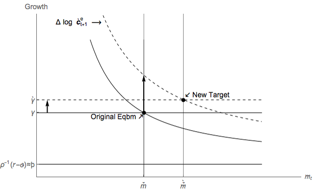
Figure 4 depicts the effects of increasing the risk of unemployment μ. The principal effect we are interested in is the upward shift in the expected consumption growth locus to Δct+1. If the household starts at the original target level of resources m, the size of the upward shift at that point is captured by the arrow originating at {m,γ}.
In the absence of other consequences of the rise in μ, the effect on the target level of m would be unambiguously positive. However, recall our adjustment to the growth rate conditional upon employment (10); this induces the shift in the income growth locus to γ which has an offsetting effect on the target m ratio. Under our benchmark parameter values, the target value of m is higher than before the increase in risk even after accounting for the effect of higher γ, but in principle it is possible for the γ effect to dominate the direct effect. Note, however, that even if the target value of m is lower, it is possible that the saving rate will be higher; this is possible because the higher γ makes a given saving rate translate into a lower ratio of wealth to income. In any case, our view is that most useful calibrations of the model are those for which an increase in uncertainty results in either an increase in the saving rate or an increase in the target ratio of resources to permanent income. This is partly because our intent is to use the model to illustate the general features of precautionary behavior, including the qualitative effects of an increase in the magnitude of transitory shocks, which unambiguously increase both target m and saving rates.
Our simple model may help explain why the attempt to estimate preference parameters like the degree of relative risk aversion or the time preference rate using consumption Euler equations has been so signally unsuccessful (Carroll, 2001). On the one hand, as illustrated in figures 3 and 4, the steady state growth rate of consumption, for impatient consumers, is equal to the steady-state growth rate of income,
On the other hand, under logarithmic utility our approximation of the Euler equation for consumption growth, obtained from equation (28), seems to tell a different story, where the last line uses the Taylor approximations used to obtain (15). The approximate Euler equation (30) does not contain any term explicitly involving income growth. How can we reconcile (29) and (30) and resolve the apparent contradiction? The answer is that the size of the precautionary term μ∇t+1 is endogenous (and depends on γ). To see this, solve (29)- (30): In steady-state, The expression in (31) helps to understand the relationship between the model parameters and the steady-state level of wealth. From figure 3 it is apparent that ∇t+1(me t) is a downward-sloping function of me t. At low levels of current wealth, much of the spending of an employed consumer is financed by current income. In the event of job loss, such a consumer must suffer a large drop in consumption, implying a large value of ∇t+1.To illustrate further the workings of the model, consider an increase in the growth rate of income. On the one hand, the right-hand side of (31) rises. But, lower wealth raises consumption risk, so that the new target level of m must be lower, and this raises the left-hand side of (31). In equilibrium, both sides of the expression rise by the same amount.
The fact that consumption growth equals income growth in the steady-state poses major problems for empirical attempts to estimate the Euler equation. To see why, suppose we had a collection of countries indexed by i, identical in all respects except that they have different interest rates ri. In the spirit of Hall (1988), one might be tempted to estimate an equation of the form
and to interpret the coefficient on ri as an empirical estimate of the value of ρ−1. This empirical strategy will fail. To see why, consider the following stylized scenario. Suppose that all the countries are inhabited by impatient workers with optimal buffer-stock target rules, but each country has a different after-tax interest rate (measured by ri). Suppose that the workers are not far from their wealth-to-income target, so that Δ log ci = γi. Suppose further that all countries have the same steady-state income growth rate and the same unemployment rate.28A regression of the form of (32) would return the estimates

Here we provide some illustrations of how the formulas derived above can be used to cleanly answer some questions that would be much more difficult to address with traditional techniques.
A substantial empirical literature attempted to measure something called ‘the interest elasticity of saving’ from Wright (1967) to the early 1980s. The inability of that literature to reach any consensus led Summers (1981) and others to turn to theoretical analysis of the problem.
As those papers showed, in a partial equilibrium infinite horizon perfect foresight context, the question ‘what is the interest elasticity of saving’ does not have a sensible answer.
In that context, an impatient consumer will run his net worth down to the sticking point defined by the maximum possible amount that he can borrow. If the impatient consumer is constrained to have a minimum wealth of zero the interest elasticity of saving well defined: It is zero, because the impatient consumer will remain at zero wealth for any variation in the interest rate such that he continues to be impatient.
The only other answer to the question (in this perfect foresight context) comes from an increase in the interest rate that switches the agent from being impatient to being patient. A consumer who is patient (relative to the prevailing interest rate) will accumulate assets forever, so in principle an arbitrarily small increment to the interest rate could (eventually) produce an arbitrarily large increase in wealth. Effectively, the interest elasticity of saving in such a case would be infinity.
It is tempting to blame these extreme results on the infinite horizon assumption. But Summers (1981) showed that while the answers obtainable from finite-horizon (life cycle) models were finite, they were still extremely – implausibly – large.
Subsequent numerical solutions showed that for specific combinations of numerical assumptions the response of saving to interest rates can be radically muted, compared to the perfect foresight benchmark. (See, e.g., Carroll (1997) or Cagetti (2001)). But such results are a leading example of the impenetrability of the numerical literature: Adepts in the literature are persuaded that the results are correct, but little intuition emerges.
In our framework, some progress can be made by thinking carefully about the results above. Define the saving rate as the amount of saving divided by market resources me i.e. the personal saving rate out of current disposable income. Saving is simply market resources minus consumption. Thus, the saving rate is given by:
| se t | =  = 1 −ce
t∕me
t = 1 −π = 1 −ce
t∕me
t = 1 −π | (33) |
where the quantity π is defined in (20).
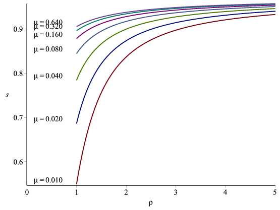
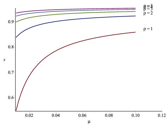
Figures 14 and 15 show the value of the target saving rate se, as the coefficient of relative risk aversion ρ and the transition probability μ are varied. Figures 16 and 17 show the value of the elasticity of the target saving rate se with respect to the interest rate R, as the coefficient of relative risk aversion ρ and the transition probability μ are varied.
The intuition for these results can be understood be thinking carefully about π: [I bet you can figure out something useful to say here!]
The tractable buffer-stock model emphasizes three factors that affect saving and that might vary substantially over time. First, because the precautionary motive decreases with wealth, the saving rate decreases as market resources m increase. Secondly, because an expansion in the availability of credit reduces the target level of wealth m, the saving rate decreases as credit conditions tighten. Thirdly, because of the precautionary saving motive, the saving rate increases as unemployment risk μ rises. Carroll, Slacalek, and Sommer (2013) estimate a structural version of the tractable model on U.S. data for the 1966-2011 period. Their main findings are: increased credit availability accounts for most of the secular decline in the saving rate; the gap between target and actual wealth accounts for the bulk of the business-cycle variation (including an important part attributable to cyclical movements in the precautionary motive).
The gist of the structural estimation can be captured by a simple, linear reduced-form model:
st = γ1 + γmmt + γceaceat + γeu 𝔼tut+4 +  X′ X′ t + 𝜖t,
 | (34) |
where market resources m are measured as the ratio of household net worth to disposable
income, lagged by one period; where cea stands for “Credit Easing Accumulated”, an
index measure of credit supply; where ut+4 is a proxy for μ based on survey responses to
four-quarter-ahead expected changes in the unemployment rate; and where the vector  t collects
other factors outside the scope of the model, e.g. demographics, corporate saving, government
saving. The theory suggests that the regression coefficients should have the following
signs:
t collects
other factors outside the scope of the model, e.g. demographics, corporate saving, government
saving. The theory suggests that the regression coefficients should have the following
signs:
| γm < 0,γcea < 0,γeu > 0, |
Table 5 reports the estimated coefficients from the univariate regression (34). The three coefficients have the predicted signs and are statistically significant. This parsimonious regression captures about 90 percent of the variation in saving.
The estimated coefficients on net wealth suggest a long-run marginal propensity to consume of about 1.2 cents out of a dollar of total wealth. This estimate is low compared to studies that do not explicitly account for credit conditions (the usual range of estimates is about 3 −7 cents). Structural estimates of the model reinforce these findings, leading Carroll, Slacalek, and Sommer (2013) to suggest that much of what the existing literature has interpreted as pure “wealth effects” may instead reflect some combination of precautionary saving and credit availability.
The high saving rates and rapid accumulation of foreign reserves in emerging economies and the associated financial imbalances between regions present economists with a number of puzzles. One interpretation of these global trends is that they reflect, in some important part, a precautionary accumulation against the risks associated with economic and financial globalization, e.g. increased exposure to external demand and supply shocks; increased vulnerability to exchange rate misalignments and sudden stops; international business cycle spillovers and contagion. Carroll and Jeanne (2009) build a small-open macroeconomy version of the tractable model of buffer-stock saving to explore some of these ideas. Individuals are matched to a job at birth, face a constant risk of permanent job-loss throughout their working life (equivalent to uncertain retirement), and die with a fixed probability independent of age. In aggregate equilibrium, labor market flows are in balance and there exists a well-defined distribution of wealth.
Among other things, Carroll and Jeanne (2009) analyze the long-run consequences of a fall in the desired stock of wealth outside of the United States. They show that domestic welfare is unambiguously reduced, in both the short and long run. The main effect operates via a decrease in the capital–output ratio: the world interest rate rises, the domestic real wage falls, stimulating exports during the transition, with the resulting stimulus to domestic output insufficient to offset the greater reduction in investment. Foreign welfare is also reduced in the long run, but may increase in the short run for those generations alive when net foreign assets accumulated by previous generations are used to finance the increase in consumption induced by the fall in the desired stock of wealth.
The core logic of our tractable model of buffer-stock saving, despite its simplicity, emerges in almost every aspect under more realistic assumptions that allow for transitory shocks, permanent shocks, and life-cycle labor-market transitions calibrated to match the details of the household income process, but after much more work (Carroll, 2016b).
We hope that the simplicity of our framework will encourage its use in analyzing questions that have so far side-stepped the role of nonfinancial risk. For example, Carroll and Jeanne (2009) construct a fully articulated model of international capital mobility for a small open economy using our buffer-stock model as the core element. We can envision a variety of other purposes the model could serve, including applications to topical questions such as the effects of risk in a search model of unemployment.
| μ ∖ρ | 1 | 2 | 3 | 4 | 5 | 6 | 7 | 8 |
| 0.01 | 2.2 | 6.8 | 11.8 | 16.5 | 20.7 | 24.5 | 28.0 | 31.1 |
| 0.02 | 3.3 | 9.2 | 15.0 | 20.0 | 24.5 | 28.5 | 32.0 | 35.2 |
| 0.04 | 5.0 | 12.2 | 18.6 | 24.1 | 28.8 | 33.0 | 36.6 | 39.7 |
| 0.08 | 7.2 | 15.6 | 22.6 | 28.4 | 33.3 | 37.6 | 41.2 | 44.4 |
| 0.16 | 9.6 | 18.8 | 26.3 | 32.4 | 37.5 | 41.8 | 45.5 | 48.7 |
| 0.32 | 11.7 | 21.4 | 29.1 | 35.5 | 40.7 | 45.1 | 48.9 | 52.2 |
| 0.64 | 13.1 | 23.1 | 31.1 | 37.5 | 42.9 | 47.4 | 51.2 | 54.5 |
| μ ∖ρ | 1 | 2 | 3 | 4 | 5 | 6 | 7 | 8 |
| 0.01 | 6.86 | 2.14 | -1.09 | -2.87 | -3.93 | -4.60 | -5.034 | -5.33 |
| 0.02 | 8.65 | 3.64 | .86 | -.71 | -1.69 | -2.35 | -2.81 | -3.13 |
| 0.04 | 9.95 | 5.38 | 3.06 | 1.67 | .74 | .07 | -.42 | -.80 |
| 0.08 | 10.76 | 7.13 | 5.24 | 4.01 | 3.13 | 2.45 | 1.92 | 1.49 |
| 0.16 | 11.21 | 8.60 | 7.08 | 6.00 | 5.17 | 4.50 | 3.96 | 3.50 |
| 0.32 | 11.46 | 9.64 | 8.40 | 7.44 | 6.66 | 6.02 | 5.48 | 5.015 |
| 0.64 | 11.58 | 10.28 | 9.22 | 8.35 | 7.62 | 7.00 | 6.47 | 6.02 |
| μ ∖ρ | 1 | 2 | 3 | 4 | 5 | 6 | 7 | 8 |
| 0.01 | .549 | .837 | .898 | .921 | .933 | .941 | .946 | .949 |
| 0.02 | .686 | .874 | .915 | .932 | .941 | .946 | .950 | .953 |
| 0.04 | .784 | .900 | .923 | .940 | .947 | .951 | .954 | .956 |
| 0.08 | .845 | .918 | .937 | .946 | .951 | .954 | .957 | .959 |
| 0.16 | .879 | .928 | .943 | .950 | .954 | .957 | .960 | .960 |
| 0.32 | .896 | .935 | .947 | .953 | .956 | .959 | .961 | .962 |
| 0.64 | .906 | .938 | .949 | .954 | .958 | .960 | .961 | .963 |
| μ ∖ρ | 1 | 2 | 3 | 4 | 5 | 6 | 7 | 8 |
| 0.01 | 4.78 | -.60 | -1.08 | -1.16 | -1.17 | -1.17 | -1.16 | -1.15 |
| 0.02 | 2.99 | -.52 | -.91 | -1.01 | -1.05 | -1.06 | -1.07 | -1.07 |
| 0.04 | 1.68 | -.48 | -.80 | -.90 | -.95 | -.97 | -.99 | -1.00 |
| 0.08 | .87 | -.47 | -.73 | -.83 | -.88 | -.91 | -.93 | -.94 |
| 0.16 | .41 | -.47 | -.69 | -.78 | -.83 | -.86 | -.89 | -.90 |
| 0.32 | .17 | -.48 | -.66 | -.75 | -.80 | -.84 | -.86 | -.88 |
| 0.64 | .046 | -.49 | -.65 | -.74 | -.79 | -.82 | -.84 | -.86 |
Estimates of the Tractable Model on Post-War U.S. Data
| |||||
| γ1 | γm | γcea | γeu | Overall | |
| 15.226 | -1.183 | -6.121 | 0.287 | ||
| (2.157) | (0.347) | (0.573) | (0.075) | ||
| 2 | 0.895 | ||||
| p–value | 0.000 | ||||
| Durbin–Watson | 0.933 | ||||
Notes : Estimation sample 1966Q2–2011Q1. Statistically significant at the 1% level.
Newey-West standard errors at 4 lags. Source : Carroll, Slacalek, and Sommer (2013).
| |||||
PT: Minor edits in the appendix, mostly presentation. Applying a second-order Taylor approximation to (13), simplifying, and rearranging yields:
The steady-state value of me, denoted m, is the solution of (19)-(21), which may be computed in
closed form. To simplify some of the intermediate steps in the algebra, define the short-hand
notation: ζ ≡ ℛκuΠ and ℛ ≡ RΓ−1 and Π ≡  1∕ρ. From this: RκuΠ = ζΓ. A series of
straightforward manipulations yields:
1∕ρ. From this: RκuΠ = ζΓ. A series of
straightforward manipulations yields:
A first point about this formula is that:
is likely to increase as μ vanishes to zero.29 Note that (36) tends to infinity as μ → 0, which implies that lim μ→0m = 1. This is precisely what would be expected since an impatient consumer is self-constrained to keep me > 1. Thus, as the risk gets infinitesimally small, the amount by which the target me exceeds its minimum possible value shrinks to zero.We now show that the RIC and GIC ensure that the denominator of the fraction in (35) is positive:

We can obtain further insight into (35) by using a judicious mix of first- and second-order Taylor expansions. Define the short-hand ψ:

Secondly, applying a first-order Taylor expansion to ψ:
Thirdly, substitute (38) into (37): PT: removed a line in the equation below (a reminder of signs of different components is not necessary here, is it?): By our definition of ω (the excess of prudence over the logarithmic benchmark):
The formula also provides insight about how the human wealth effect works in equilibrium. All else equal, the human wealth effect is captured by the (γ −r) term in the denominator of (41): it is obvious that a larger value of γ results in a smaller target value for m. However, the size of the human wealth effect also depends on the magnitude of the patience and prudence contributions to the denominator, and those terms could dominate the human wealth effect.
For (41) to make sense, we need the denominator of the fraction to be positive. Let:

The same set of derivations imply that we can replace the denominator in (41) with the negative of the RHS of (43), yielding a more compact expression for the target level of resources:
This formula makes plain that an increase in either form of impatience raises the denominator of the fraction in (44) and thus reduces the target level of assets.Two specializations of the formula are particularly useful. The first useful special case is ρ = 1 (logarithmic utility). In this case,

The second useful special case is r = 𝜗 (but ρ > 1). In this case,

| a | - | end-of-period t assets (after consumption decision) |
| b | - | middle-of-period t balances (before consumption decision) |
| c | - | consumption |
| ℓ | - | personal labor productivity |
| m | - | market resources (capital, capital income, and labor income) |
| R, r | - | interest factor, rate |
| W | - | aggregate wage |
| G | - | growth factor for aggregate wage rate W |
| Γ ≡ G∕(1 −μ) | - | conditional (on employment) growth factor for individual labor income |
| γ | - | log Γ, conditional growth rate for labor income |
| β | - | time preference factor (= 1∕(1 + 𝜗)) |
| ξ | - | dummy variable indicating the employment state, ξ ∈ {0,1} |
| κ | - | marginal propensity to consume |
| ρ | - | coefficient of relative risk aversion |
| 𝜗 | - | time preference rate (≈ −log β) |
| μ | - | probability of falling into permanent unemployment |
| Þ, þ | - | absolute patience factor, rate |
| ÞΓ, þγ | - | growth patience factor, rate |
| ÞR, þr | - | return patience factor, rate |
| ω | - | excess prudence factor (= (ρ −1)∕2) |
| ∇ | - | proportional consumption drop upon entering unemployment |
| ℛ | - | short for R∕Γ |
Aiyagari, S. Rao (1994): “Uninsured Idiosyncratic Risk and Aggregate Saving,” Quarterly Journal of Economics, 109, 659–684.
Barsky, Robert B., F. Thomas Juster, Miles S. Kimball, and Matthew D. Shapiro (1997): “Preference parameters and behavioral heterogeneity: An experimental approach in the health and retirement study*,” Quarterly Journal of Economics, 112(2), 537–579, http://www.jstor.org/stable/2951245.
Becker, Robert A., and C. Foias (1987): “A Characterization of Ramsey Equilibrium,” Journal of Economic Theory, 41(1), 173–184.
Berk, Jonathan, Richard Stanton, and Josef Zechner (2009): “Human Capital, Bankruptcy, and Capital Structure,” Manuscript, Hass School of Business, Berkeley.
Bernanke, Benjamin, Mark Gertler, and Simon Gilchrist (1996): “The Financial Accellerator and the Flight to Quality,” Review of Economics and Statistics, 78, 1–15.
Bewley, Truman (1977): “The Permanent Income Hypothesis: A Theoretical Formulation,” Journal of Economic Theory, 16, 252–292.
Cagetti, Marco (2001): “Interest Elasticity in a Life-Cycle Model with Precautionary Savings,” The American Economic Review, 91(2), pp.418–421.
____________ (2003): “Wealth Accumulation Over the Life Cycle and Precautionary Savings,” Journal of Business and Economic Statistics, 21(3), 339–353.
Carroll, Christopher (2016a): “Theoretical Foundations of Buffer Stock Saving,” Manuscript, Department of Economics, Johns Hopkins University, Available at http://econ.jhu.edu/people/ccarroll/papers/BufferStockTheory.
Carroll, Christopher D. (1992): “The Buffer-Stock Theory of Saving: Some Macroeconomic Evidence,” Brookings Papers on Economic Activity, 1992(2), 61–156, http://econ.jhu.edu/people/ccarroll/BufferStockBPEA.pdf.
____________ (1997): “Buffer Stock Saving and the Life Cycle/Permanent Income Hypothesis,” Quarterly Journal of Economics, CXII(1), 1–56, http://econ.jhu.edu/people/ccarroll/BSLCPIH.zip.
____________ (2001): “Death to the Log-Linearized Consumption Euler Equation! (And Very Poor Health to the Second-Order Approximation),” Advances in Macroeconomics, 1(1), Article 6, http://econ.jhu.edu/people/ccarroll/death.pdf.
____________ (2016b): “Theoretical Foundations of Buffer Stock Saving,” manuscript, Department of Economics, Johns Hopkins University, Available at http://econ.jhu.edu/people/ccarroll/papers/BufferStockTheory.
Carroll, Christopher D., and Olivier Jeanne (2009): “A Tractable Model of Precautionary Reserves, Net Foreign Assets, or Sovereign Wealth Funds,” NBER Working Paper Number 15228, http://econ.jhu.edu/people/ccarroll/papers/cjSOE.
Carroll, Christopher D., and Miles S. Kimball (1996): “On the Concavity of the Consumption Function,” Econometrica, 64(4), 981–992, http://econ.jhu.edu/people/ccarroll/concavity.pdf.
Carroll, Christopher D., Jiri Slacalek, and Martin Sommer (2013): “Dissecting Saving Dynamics: Measuring Wealth, Precautionary, and Credit Effects,” Manuscript, Johns Hopkins University, http://econ.jhu.edu/people/ccarroll/papers/cssUSSaving/.
Chamberlain, Gary, and Charles A. Wilson (2000): “Optimal Intertemporal Consumption Under Uncertainty,” Review of Economic Dynamics, 3(3), 365–395.
Clarida, Richard H. (1987): “Consumption, Liquidity Constraints, and Asset Accumulation in the Face of Random Fluctuations in Income,” International Economic Review, XXVIII, 339–351.
Fisher, Irving (1930): The Theory of Interest. MacMillan, New York.
Friedman, Milton A. (1957): A Theory of the Consumption Function. Princeton University Press.
Gourinchas, Pierre-Olivier, and Jonathan Parker (2002): “Consumption Over the Life Cycle,” Econometrica, 70(1), 47–89.
Hall, Robert E. (1988): “Intertemporal Substitution in Consumption,” Journal of Political Economy, XCVI, 339–357, Available at http://www.stanford.edu/~rehall/Intertemporal-JPE-April-1988.pdf.
Jagannathan, Ravi, Keiichi Kubota, and Hitoshi Takehara (1998): “Relationship between Labor-Income Risk and Average Return: Empirical Evidence from the Japanese Stock Market,” Journal of Business, 71(3), 319–47.
Kimball, Miles S. (1990): “Precautionary Saving in the Small and in the Large,” Econometrica, 58, 53–73.
Krusell, Per, and Anthony A. Smith (1998): “Income and Wealth Heterogeneity in the Macroeconomy,” Journal of Political Economy, 106(5), 867–896.
Markowitz, Harold (1959): Portfolio Selection: Efficient Diversification of Investment. John Wiley and Sons, New York.
Merton, Robert C. (1969): “Lifetime Portfolio Selection under Uncertainty: The Continuous Time Case,” Review of Economics and Statistics, 50, 247–257.
Parker, Jonathan A., and Bruce Preston (2005): “Precautionary Saving and Consumption Fluctuations,” American Economic Review, 95(4), 1119–1143.
Phelps, Edward S. (1960): “The Accumulation of Risky Capital: A Sequential Utility Analysis,” Econometrica, 30(4), 729–743.
Ramsey, Frank (1928): “A Mathematical Theory of Saving,” Economic Journal, 38(152), 543–559.
Samuelson, Paul A. (1969): “Lifetime Portfolio Selection by Dynamic Stochastic Programming,” Review of Economics and Statistics, 51, 239–46.
Schechtman, Jack, and Vera Escudero (1977): “Some results on ‘An Income Fluctuation Problem’,” Journal of Economic Theory, 16, 151–166.
Sethi, S.P., and G.L. Thompson (2000): Optimal Control Theory: Applications to Management Science and Economics. Kluwer Academic Publishers, Boston.
Summers, Lawrence H. (1981): “Capital Taxation and Accumulation in a Life Cycle Growth Model,” American Economic Review, 71(4), 533–544, http://www.jstor.org/stable/1806179.
Tobin, James (1958): “Liquidity Preference as Behavior Towards Risk,” Review of Economic Studies, XXXV(67), 65–86.
Toche, Patrick (2005): “A Tractable Model of Precautionary Saving in Continuous Time,” Economics Letters, 87(2), 267–272, http://ideas.repec.org/a/eee/ecolet/v87y2005i2p267-272.html.
Uzawa, Hirofumi (1968): “Time Preference, the Consumption Function, and Optimum Asset Holdings,” in Value, Capital, and Growth: Papers in Honor of Sir John Hicks, ed. by J. N. Wolfe, pp. 485–504. Edinborough University Press, Chicago.
Wright, Colin (1967): “Some Evidence on the Interest Elasticity of Consumption,” The American Economic Review, 57(4), pp.850–855.
Zeldes, Stephen P. (1989): “Optimal Consumption with Stochastic Income: Deviations from Certainty Equivalence,” Quarterly Journal of Economics, 104(2), 275–298.


![( e ) ( e ) { [( e )ρ ]} 1∕ρ
ct+1Γ- = ct+1- = ÞÞÞ 1 + μ ct+1- − 1 , (13)
cet cet cut+1](ctDiscrete15x.svg)


![[(ce )ρ ]
(ÞÞÞ ∕Γ )−ρ = 1 + μ -tu+1 − 1
ct+1
ce [(ÞÞÞ∕Γ )−ρ − (1 − μ)]1∕ρ
⇒ -u = ----------------- . (17)
c μ](ctDiscrete20x.svg)
![u e e
m t+1 = R (m[ t − ct) ]
--mut+1-- -met- -cet-- --Wtℓt--
⇒ W ℓ = R W ℓ − W ℓ W ℓ
t+1 t+u1 et te t t t+1 t+1
⇒ m t+1 = R (m t − ct)∕Γ
⇒ cut+1 = κuR (met − cet)∕Γ
u e e u
⇒ c = (m − c)κ R ∕Γ (18)](ctDiscrete21x.svg)

![[ ]
--π-- u (ÞÞÞ∕Γ-)−ρ-−-(1 −-μ)-1∕ρ
1 − π ≡ κ (R ∕Γ ) μ . (20)](ctDiscrete23x.svg)


![( e ) { [( e )ρ ]}1∕ρ
ct+1- = ÞÞÞ 1 + μ ct+1- − 1 . (28)
cet cut+1](ctDiscrete33x.svg)


![{ [(ce )ρ ]}1∕ρ { [(cu + ce − cu )ρ ]} 1∕ρ
1 + μ -t+1 − 1 = 1 + μ -t+1---t+1----t+1 − 1
cut+1 cut+1
= {1 + μ [(1 + ∇ )ρ − 1]}1∕ρ
{ [ t+1 ]}1∕ρ
≈ 1 + μ 1 + ρ∇t+1 + ρ(∇t+1)2ω − 1
{ }1∕ρ
= 1 + ρμ(∇t+1 + (∇t+1)2ω)
≈ 1 + μ (1 + ∇t+1ω )∇t+1.](ctDiscrete43x.svg)


