A Tractable Model of Precautionary Reserves,
Net Foreign Assets, or Sovereign Wealth Funds
February 2019
| Christopher D. Carroll 1 |
| . |
| Olivier Jeanne 2 |
| . |
_____________________________________________________________________________________
Abstract
We model the motives for residents of a country to hold foreign assets, including the
precautionary motive that has been omitted from much previous literature as intractable. Our model
captures the principal insights from the existing literature on the precautionary motive with a novel
and convenient formula for the economy’s target asset ratio. The target is the value of assets that
balances growth, impatience, prudence, risk, intertemporal substitution, and the rate of return. We
use the model to shed light on two topical questions: “Upstream” flows of capital from developing to
advanced countries, and the long-run impact of resorbtion of global financial imbalances.
Buffer Stock Saving, Net Foreign Assets, Sovereign Wealth Funds, Foreign Exchange Reserves, Small Open Economy
C61
| PDF: | http://econ.jhu.edu/people/ccarroll/papers/cjSOE.pdf |
| Slides: | http://econ.jhu.edu/people/ccarroll/papers/cjSOE-Slides.pdf |
| Web: | http://econ.jhu.edu/people/ccarroll/papers/cjSOE/ |
| Repo: | https://github.com/llorracc/cjSOE |
| Code: | http://econ.jhu.edu/people/ccarroll/code/Tractable.zip |
| (Contains code solving this paper’s model (and related models)) |
1Carroll: ccarroll@jhu.edu, Department of Economics, 440 Mergenthaler Hall, Johns Hopkins University, Baltimore, MD 21218, http://econ.jhu.edu/people/ccarroll/, and National Bureau of Economic Research. 2Jeanne: ojeanne@jhu.edu, Department of Economics, 440 Mergenthaler Hall, Johns Hopkins University, Baltimore, MD 21218, http://econ.jhu.edu/people/jeanne/, and National Bureau of Economic Research.
The remarkable accumulation of foreign reserves in emerging economies has captured the attention of academics, policymakers, and financial markets, partly because reserve accumulation seems to have played a role in the development of global financial imbalances. A distinct (but probably related) puzzle is that national saving rates of fast-growing emerging economies have been rising over time,2 leading to surprising “upstream” flows of capital from developing to rich countries. The corresponding accumulation of foreign assets in “sovereign wealth funds” has also attracted scrutiny as those funds have emerged as prominent actors in global capital markets.
A popular interpretation of all these trends is that they reflect precautionary saving against the risks associated with economic globalization.3
Such an interpretation raises several questions. What are the main determinants of the demand for external assets? What are the welfare benefits of international integration, if it leads developing countries to export rather than import capital? How persistent will the increase in developing countries’ demand for foreign assets prove to be? How does the precautionary motive for asset accumulation interact with other, better-understood motives?
This paper introduces a tractable model that can be used to analyze these questions (and others). Our model is a small-open-macroeconomy version of the model of individual precautionary saving developed by Carroll (2016a), based on Toche (2005). With it, we characterize the dynamics of foreign asset accumulation using phase diagrams that should be readily understandable to anyone familiar with the benchmark Ramsey model of economic growth, and we derive closed-form expressions that relate the target level of net foreign assets to fundamental determinants like the degree of risk, the time preference rate, and expected productivity growth. The model’s structure is simple enough to permit straightforward calculations of welfare-equivalent tradeoffs between growth, social insurance generosity, and risk.
We then present two applications of our framework.
First, we look at what the model says about the puzzling relation between economic growth and international capital flows (especially the fact that fast-growing developing countries tend to export capital). Several recent papers (e.g., Chamon, Liu, and Prasad (2010) and Wen (2009)) argue in particular that the rise in China’s saving rate reflects precautionary motives. We show that merely adding precautionary saving to the usual intertemporal optimization framework does not reverse that model’s implication that exogenously higher growth should cause lower saving. But the growth-to-saving puzzle can be explained in our framework if the bargain that countries make when they embark on a path of rapid development involves not only a pickup in productivity growth but also an increase in the degree of idiosyncratic risk borne by individuals (like unemployment spells that result in substantial lost wages).4
Second, we use a two-country version of the model to investigate the long-term impact on the United States and the rest of the world if the recent global financial imbalances were to be resorbed by a fall in non-U.S. savings (as some analysts have urged). Our model implies that a decrease in the desired level of wealth in the rest of the world has a substantial negative impact on the global capital stock as well as the U.S. (and global) real wage.
A central purpose of the paper is to distill the main insights of the complex literature that interprets capital flows through the lens of the precautionary motive. We aim to improve on an older literature on the ‘intertemporal approach to the current account’ that simply ignores precautionary behavior by considering a linear-quadratic formulation of the consumption-saving problem (see Obstfeld and Rogoff (1995) for a review).5
More recently, one strand of the intertemporal literature looks at the effects of aggregate risk on domestic precautionary wealth. For example, Durdu, Mendoza, and Terrones (2009) present some estimates of the optimal level of precautionary wealth accumulated by a small open economy in response to business cycle volatility, financial globalization, and the risk of a sudden stop in credit. They conclude that these risks are plausible explanations of the observed surge in reserves in emerging market countries.6 Arbatli (2008) argues that precautionary motives associated with the possibility of sudden stops can explain the dynamics of the current account in emerging economy business cycles. Fogli and Perri (2006) instead take the perspective of the U.S. and argue that the decrease in its saving rate can be explained partly by the moderation in the volatility of its business cycle.
Closer to our paper are the contributions that examine the impact of idiosyncratic risk on saving behavior. Mendoza, Quadrini, and Ríos-Rull (2009) model the determination of capital flows in a closed world in which economies differ by their level of financial development (market completeness). They find that international financial integration can lead to the accumulation of a large level of net and gross liabilities by the more financially advanced region. Sandri (2014) presents a model in which growth acceleration in a developing country causes a larger increase in saving than in investment because capital market imperfections induce entrepreneurs not only to self-finance investment but also to accumulate precautionary wealth outside their business enterprise. Another recent contribution is by Angeletos and Panousi (2011), who adapt a Merton (1969)-Samuelson (1969) model of portfolio choice to a general equilibrium context in which the risky asset, in each country, is interpreted as reflecting returns to entrepreneurial activity with an undiversifiable risky component. They calibrate the degree of financial development by the magnitude of the undiversifiable component of entrepreneurial risk. When a regime change suddenly allows international mobility of the riskless asset in their model, the result is an immediate large reallocation of risky capital from the less to the more developed economy.7
The recent literature offers several explanations for the accumulation of foreign assets in high-growth emerging market economies that involve financial frictions other than the lack of insurance against income risk. For example, Caballero, Farhi, and Gourinchas (2008) suggest that those flows have been driven by countries’ supply of (rather than demand for) assets. Song, Storesletten, and Zilibotti (2011) present a model in which capital flows upstream from a high-growth country because of a friction in the intermediation of domestic saving. Aguiar and Amador (2011) explain the capital outflows by the accumulation of foreign exchange reserves that are posted as a “bond" to prevent the expropriation of investors. Coeurdacier, Guibaud, and Jin (2015) show that in an open-economy model with overlapping generations, the interaction between growth differentials and household credit constraints can explain the divergence in private saving rates between advanced and emerging economies. Bacchetta and Benhima (2015) present a model in which firms in a high-growth economy are credit-constrained and need to accumulate funds in order to finance working capital (see also Buera and Shin (2009) for a similar mechanism).
Also related is recent work by Barro (2006), reviving the proposal of Rietz (1988) that the equity premium puzzle can be explained by a fear of rare but catastrophic events. Our model’s risk is to the consumer’s labor income rather than to an investor’s financial returns, but our framework shares the intuition that precautionary behavior against occasional disasters is powerful even in periods when the disasters are not observed.
Several of our analytical results resonate with themes developed quantitatively (or at least touched upon) in the papers cited above (in particular, the importance of domestic financial development or social insurance for international capital flows). The main comparative advantages of our analysis are three. First, the insights are reflected in tractable analytical formulas. The impact of key variables can be analyzed using a simple diagram or closed-form expressions—although (as usual) analysis of transitional dynamics requires numerical solution tools (which we provide).8 Second, our model of prudent (Kimball (1990)) intertemporal choice is integrated with a standard neoclassical treatment of production (Cobb-Douglas with labor augmenting productivity growth), so that the familiar Ramsey-Cass-Koopmans framework can be viewed as the perfect-insurance special case of our model. This allows us analyze the link between economic development and capital flows in a way that is directly comparable to the corresponding analysis in the standard model.9 Finally, we do not believe that a model of China’s (or Japan’s, or Korea’s) high saving can be fully persuasive without explicitly tackling the relationship of increased saving to rapid economic growth. The financial flows from developing to developed countries in Mendoza, Quadrini, and Ríos-Rull (2009) are not related to growth (which is identical in the respective economies), while in Sandri (2014) the saving is entirely in the entrepreneurial sector (as in Angeletos and Panousi (2011)), although empirical evidence suggests that much of the recent increase in saving in China has come from the household sector (Song and Yang (2010)), a finding that is consistent with the earlier experience in Japan and other countries.
We consider a small open economy whose population and productivity grow at constant rates. A resident of this economy accumulates precautionary wealth in order to insure against the risk of unemployment, which results in complete and permanent destruction of the individual’s human capital.10 ,11 The saving decisions of our individuals aggregate to produce “net foreign assets” for the economy as a whole.12
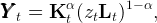
Domestic output is produced according to the usual Cobb-Douglas function:
|
| (1) |
where Kt is domestic capital and Lt is the supply of domestic labor. The productivity of labor increases by a constant factor G in every period,
 |
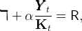
Capital and labor are supplied in perfectly competitive markets. Capital is perfectly mobile internationally, so that the marginal return to capital is the same as in the rest of the world,
 | (2) |
where the Hebrew letter daleth ℸ ≡ (1 − δ) is the proportion of capital that remains undepreciated after production, and R is the worldwide constant risk-free interest factor. Thus, the capital-to-output ratio is constant and equal to
 | (3) |
Labor is supplied by domestic workers. Each worker is part of a ‘generation’ born at the same date, and every new generation is larger by the factor Ξ than the newborn generation in the previous period. If we normalize to 1 the size of the generation born at t = 0, the generation born at t will be of size Ξt.
An individual’s life has three phases: Employment, followed by unemployment,
which terminates in death. Transitions to unemployment and to death follow
Poisson processes with constant arrival rates. The probability that an employed
worker will become unemployed is ℧ (while the probability of remaining
employed is denoted as the cancellation of unemployment,  ≡ 1 − ℧). The
probability that an unemployed individual dies before the next period is D; the
probability of survival is cancellation of the probability of death,
≡ 1 − ℧). The
probability that an unemployed individual dies before the next period is D; the
probability of survival is cancellation of the probability of death,  ≡ 1 −D.
(Individuals are permitted to die only after they have become unemployed.) The
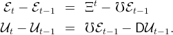
employed population, ℰ, and the unemployed population, 𝒰 thus satisfy the
dynamic equations,
≡ 1 −D.
(Individuals are permitted to die only after they have become unemployed.) The
employed population, ℰ, and the unemployed population, 𝒰 thus satisfy the
dynamic equations,
Total labor supply is the number of workers times the average labor supply per worker,
 | (4) |
(1) and (3) together imply that in the balanced growth equilibrium capital and output grow by the same factor ΞG in every period. Finally, the real wage is equal to the marginal product of labor,
 |
which grows by the factor G in every period.
Perfect capital mobility means that residents and non-residents can hold domestic capital, and can hold foreign assets or issue foreign liabilities. Our main variable of interest is Nt, the aggregate net foreign assets of the economy at the end of period t. As a matter of accounting, the country’s net foreign asset position is equal to the difference between the value of its total wealth and the value of domestic physical capital,
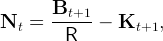 | (5) |
where Bt+1∕R is the present discounted value at the end of period t of next period’s total wealth (see Appendix A.2 for the basic national accounting relationships in this economy). The dynamics of Bt are determined by the consumption/saving choices of individuals, to which we now turn.
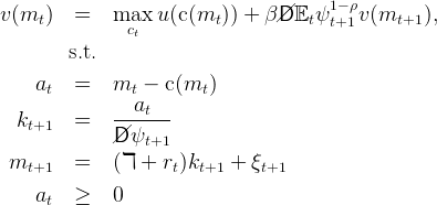
Using lower-case variables for individuals, the period-t budget constraint relates current consumption c to current labor income and current and next-period’s wealth b,13
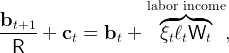 | (6) |
where ξ is a dummy variable indicating the consumer’s employment state. Everyone in this economy is either employed (state ‘e’), in which case ξ = 1, or unemployed (state ‘u’), in which case ξ = 0, so that for unemployed individuals labor income is zero.
The labor productivity ℓ of each individual worker who remains employed is assumed to grow by a factor X every period because of increasing eXperience,
 | (7) |
where ℓ0 is the labor supply of a newborn individual. X can be interpreted as the factor that governs the rate at which an individual’s work skills improve, perhaps as a result of human capital accumulation, whereas G is the factor by which productivity grows in the economy as a whole, perhaps due to societal knowledge accumulation and technological advance (Mankiw (1995)). This means that for a consumer who remains employed, labor income will grow by factor

Following Toche (2005), unemployment entails a complete and permanent destruction of the individual’s human wealth: Once a person becomes unemployed, that person can never be employed again. Thus, unemployment could also be interpreted as retirement (we calibrate the model so that the average length of the working life is forty years). Employed consumers face a constant risk ℧ of becoming unemployed regardless of their age.
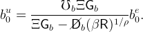
Consumers have a CRRA felicity function u(∙) = ∙1−ρ∕(1 − ρ) and discount future utility geometrically by β per period. We assume that unemployed workers have access to life insurance à la Blanchard (1985) and can convert their wealth into annuities. As shown in the appendix, the solution to the unemployed consumer’s optimization problem is
 | (8) |
where the u superscript now signifies the consumer’s (un)employment status, and κu, the marginal propensity to consume for the perfect foresight unemployed consumer, is given by
We assume κu > 0, which is necessary for the unemployed consumer’s problem to have a well-defined solution.Following Carroll (2016b), it will be useful to define a ‘growth patience factor’:
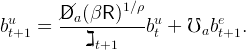
which is the factor by which ce would grow in the perfect foresight version of the model with labor income growth factor Γ. We will assume that the growth patience factor ÞΓ is less than one This condition—which Carroll (2016b) dubs the ‘perfect foresight growth impatience condition’ (PF-GIC)—ensures that a consumer facing no uncertainty is sufficiently impatient that his wealth-to-permanent-income ratio will fall over time.The Euler equation for an employed worker is
 |
Now define nonbold variables as the boldface equivalent divided by the level of permanent labor income for an employed consumer, e.g. cet = cet∕(Wtℓt), and rewrite the consumption Euler equation as
 | (12) |
while the budget constraint of an employed worker can be written, in normalized form, as
 | (13) |
Using this equation and cut+1 = κubet+1 to substitute out cut+1 from (12) (since a worker who becomes unemployed in period t + 1 starts with wealth bt+1e), we have
![[ ( e ) ρ]− 1∕ρ
e /1∕ρ e ÞÞÞ-Γ---------ct---------
ct+1 = ÞÞÞ Γ /℧ c t 1 − ℧ κu R ∕ Γ (be − ce+ 1 ) .
t t](cjSOE21x.png) | (14) |
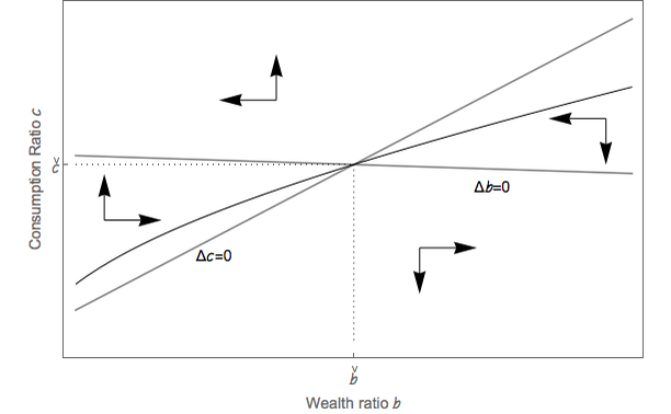
Equations (13) and (14) characterize the dynamics for the pair of variables
(bet,cet). It is possible to show (see the appendix) that those dynamics are
saddle-point stable, and that the ratio of wealth to income, bte, converges toward
a positive limit, the target wealth-to-income ratio, denoted by  e
. Figure 1
presents the phase diagram.
e
. Figure 1
presents the phase diagram.
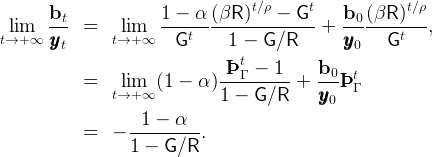
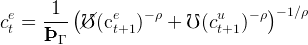
We now determine the long-run target wealth-to-income ratio. Setting
cet+1 = cet = č and cut+1 = κ in equation (12) gives
 | (15) |
and setting bet+1 = bet =  and cet = č in equation (13) gives,
 | (16) |
Eliminating č between (15) and (16) then gives an explicit formula for the target wealth-to-income ratio,
![[ ( − ρ )1 ∕ρ] − 1
Γ u ÞÞÞ Γ − 1
ˇb = -- − 1 + κ 1 + ---------- .
R ℧](cjSOE27x.png) | (17) |
Here is the intuition behind the target wealth ratio: On the one hand, consumers are growth-impatient, which prevents their wealth-to-income ratio from heading off to infinity. On the other hand, consumers have a precautionary motive that intensifies more and more as the level of wealth gets lower and lower. At some point as wealth declines, the precautionary motive gets strong enough to counterbalance impatience. The point where impatience matches prudence defines the target wealth-to-income ratio.
Expression (17) encapsulates several of the key economic effects captured by the model. The human wealth effect of growth is captured by the Γ and ÞΓ terms. Increasing Γ will decrease the growth patience factor ÞΓ and therefore reduce the target level of wealth. An increase in the worker’s patience (an increase in β and in the growth patience factor ÞΓ) boosts the target level of wealth. Finally, an increase in unemployment risk increases the target level of precautionary wealth.14 Those comparative statics results can be summarized as
The response of the target asset ratio to the risk aversion parameter ρ is less
straightforward. On the one hand, higher risk aversion enhances the demand for
precautionary reserves. On the other hand, it also implies that consumption is
less elastic intertemporally. The response of  e
to R is also ambiguous, which is
unsurprising given that even in the deterministic model the relation between
interest rates and spending can be either positive or negative depending on the
relative sizes of the income, subsititution, and human wealth effects. In
our model it is possible to show that if ρ ≤ 1, then the target level the
wealth-to-income ratio increases with the interest rate. For the usual case where
ρ > 1, however, the sign of the response of
e
to R is also ambiguous, which is
unsurprising given that even in the deterministic model the relation between
interest rates and spending can be either positive or negative depending on the
relative sizes of the income, subsititution, and human wealth effects. In
our model it is possible to show that if ρ ≤ 1, then the target level the
wealth-to-income ratio increases with the interest rate. For the usual case where
ρ > 1, however, the sign of the response of  e
to R could be positive or
negative.
e
to R could be positive or
negative.
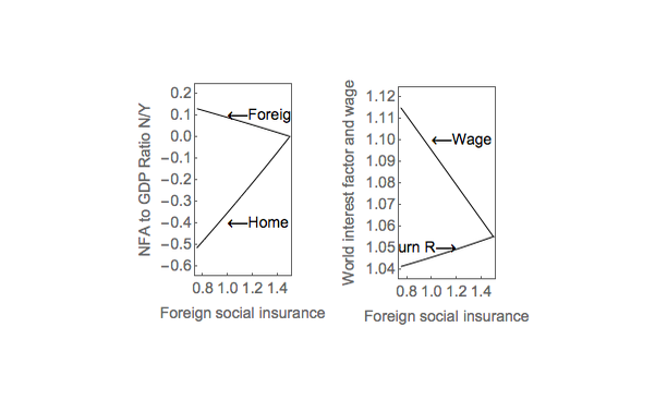
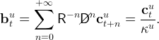
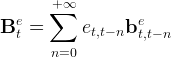
We now add up the individuals’ balance sheets to find the country’s aggregate net foreign assets. We first present a general formula that aggregates the resources of all generations of employed and unemployed workers. We then specialize this formula under two assumptions about the initial ‘stake’ of newborns in the economy. (A ‘stake’ is a transfer received by newborns). In the model without stakes, newborns do not receive any transfer and must accumulate wealth through their own frugality. Their microeconomic problem, therefore, is the one we have described in the previous section. In the model with stakes, newborns receive a transfer that puts their wealth-to-income ratio at par with the rest of the population. The main advantage of the model with stakes is that it is more tractable and yields a closed-form expression for the ratio of net foreign assets to GDP.
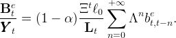
First, we focus on the wealth of the employed households. Calculations in the appendix show that the ratio of employed workers’ wealth to output is given by
where bet,t−n is the wealth-to-income ratio at t of the workers born at t−n, and Λ is the factor by which the share of a generation in total labor supply shrinks every period. Equation (19), thus, says that the ratio of workers’ wealth to output is the average of the individual wealth-to-labor-income ratios over the past generations, weighted by the share of each generation in total labor supply and by the share of labor income in total output (1 − α).Second, consider the wealth of the unemployed households (managed by the Blanchardian life insurance company). The aggregate wealth of unemployed households satisfies the dynamic equation,
 |
where the first term on the right-hand side reflects the accumulation of wealth by the previously-unemployed households, and the second term is the wealth of newly-unemployed households. The unemployed households consume a constant fraction of their wealth, Cut = κuBut, so that the equation above can be rewritten,
 | (20) |
This equation fully characterizes the dynamics of the unemployed households’ wealth ratio for a given path for the employed workers’ wealth ratio.
Now we consider a steady state in which the wealth of the employed is a
constant fraction of GDP, Be = Be∕ . Then equation (20) and
  t+1∕
t+1∕ t = ΞG
imply that the ratio of wealth to GDP is also constant for unemployed
households,15
t = ΞG
imply that the ratio of wealth to GDP is also constant for unemployed
households,15
 | (21) |
The ratio of net foreign assets to GDP is obtained by subtracting domestic
capital from domestic wealth. Using (3), (5), (21),  t+1∕
t+1∕ t = ΞG, and
Bt = Bet + But, the ratio of net foreign assets to GDP is given by
t = ΞG, and
Bt = Bet + But, the ratio of net foreign assets to GDP is given by
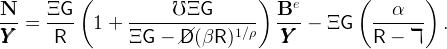 | (22) |
This expression gives the country’s ratio of net foreign assets to GDP in terms of
the exogenous parameters and one endogenous variable, the ratio of employed
workers’ wealth to GDP, Be∕ . We now present two ways of pinning down the
value of this endogenous variable.
. We now present two ways of pinning down the
value of this endogenous variable.
The most natural assumption is that newborns enter the economy with zero wealth, and must save some of their income to ensure that they do not starve if they become unemployed. In this case, analysis must be performed using simulation methods, because households of different ages will have different ratios of wealth to income. (With a concave and nonanalytical consumption function, analytical aggregation cannot be performed.)
In this version of the model, each individual is faced with exactly the same problem as in section 2.2. We denote by be(n) the level of normalized wealth held at the beginning of period n of the individual’s life in the problem of section 2.2. We assume that the individual starts his life with zero wealth, be(0) = 0. In other words, be(n)n=0,1,2,.. is the optimal time path of the individual’s wealth. Then we can replace bet,t−n by be(n) in equation (19),
The ratio of workers’ wealth to GDP is constant, and can be computed numerically based on the path be(n)n=0,1,.... Note that this ratio is lower than (1 − α) e
, since it is a weighted average of (1 − α)be(n), which converge toward
(1 − α)
e
, since it is a weighted average of (1 − α)be(n), which converge toward
(1 − α) e
from below.
e
from below.
We now consider a version of the model in which an exogenous redistribution program guarantees that the behavior of employed households can be understood by analyzing the actions of a “representative employed agent.” This will be achieved by the introduction of lump-sum transfers that ensure that the newborn individuals are endowed with the same wealth-to-income ratio that older generations already hold. This is explicitly not an inheritance, as we have assumed that individuals have no bequest motive and newborns are unrelated to anyone in the existing population. Our motivation is largely to make the model more tractable, rather than to represent an important feature of the real world; hence, we perform simulations designed to show that the characteristics of the model with no ‘stake’ are qualitatively and quantitatively similar to those of the more tractable model with a carefully chosen ‘stake.’
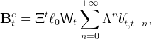
The details of the model with stakes are given in the appendix. The transfer ensures that the workers have the same wealth-to-income ratio at all times. Thus one can replace bet,t−n by bet in equation (19), which gives,
 | (24) |
where Bet follows the same saddle-point dynamics as for a single agent (adjusted for the transfer).
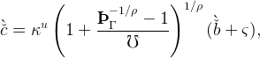
In the long run (see the appendix), bet converges to
![[ ( − ρ )1 ∕ρ] − 1
ˇ Γ 1 u ÞÞÞΓ − 1
ˇb = --− ------- + κ 1 + ----------
R 2 − Λ ℧](cjSOE48x.png) | (25) |
so that (25) implies a closed-form expression for the ratio of workers’ wealth to GDP,
This expression can be plugged into equation (22) to find the ratio of net foreign assets to GDP. It is interesting to compare formula (25) with the one that we obtained for an
individual in the model without stakes—equation (17). Since Λ < 1 we have
 <
<  . Thus equations (17) and (25) both predict that the ratio of wealth to
GDP is lower than (1 − α)
. Thus equations (17) and (25) both predict that the ratio of wealth to
GDP is lower than (1 − α) , but in the new formula this comes from the
fact that the target wealth-to-income ratio is lowered by the tax, rather
than from the fact that the wealth-to-income ratio is lower for younger
workers.
, but in the new formula this comes from the
fact that the target wealth-to-income ratio is lowered by the tax, rather
than from the fact that the wealth-to-income ratio is lower for younger
workers.
We will show below that the model with stakes provides a good approximation to the model with no stake. But the model with stakes has several advantages. First, the transition dynamics can be characterized using equation (26). In the model without stakes the transition dynamics involve an infinite state space as the wealth-to-income ratio must be tracked separately for each generation. Second, the model with stakes gives a closed-form expression for the steady state ratio of foreign assets to GDP. This makes it possible to study analytically how the ratio of foreign assets to GDP depends on the exogenous parameters of the model. With formula (23), by contrast, such a study must rely on numerical simulations.
Our benchmark calibration is reported in Table 1. The value for the unemployment probability, ℧, implies that a newborn worker expects to be employed for 40 years. The value for the probability of death, D, implies that the expected lifetime of a newly unemployed worker is 20 years.
| α | ℸ | Ξ | G | R | β−1 | X | ℧ | ρ | D |
| 0.3 | 0.94 | 1.01 | 1.04 | 1.04 | 1.04 | 1.01 | 0.025 | 2 | 0.05 |
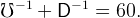
The long-run levels of be and ce are given by  = 4.85 and č = 0.95. The time
paths for bet and cet are shown in Figure 2. The convergence to the targets is
relatively rapid. The individual saves more than one third of his income on
average in the first ten years of his life, after which his wealth-to-income ratio
already exceeds two thirds of the target level. The wealth-to-income ratio reaches
99 percent of the target level after 40 years (the average duration of
employment).
= 4.85 and č = 0.95. The time
paths for bet and cet are shown in Figure 2. The convergence to the targets is
relatively rapid. The individual saves more than one third of his income on
average in the first ten years of his life, after which his wealth-to-income ratio
already exceeds two thirds of the target level. The wealth-to-income ratio reaches
99 percent of the target level after 40 years (the average duration of
employment).
For the benchmark calibration we find: K∕ = 3, N∕
 = 0.420 in the model
with no stakes, and N∕
= 0.420 in the model
with no stakes, and N∕ = 0.719 in the model with stakes. These levels have
the right order of magnitude (in view of the fact that most countries have a ratio
of foreign assets to GDP between minus and plus 100 percent of GDP, based on
the database of Lane and Milesi-Ferretti (2007)).
= 0.719 in the model with stakes. These levels have
the right order of magnitude (in view of the fact that most countries have a ratio
of foreign assets to GDP between minus and plus 100 percent of GDP, based on
the database of Lane and Milesi-Ferretti (2007)).
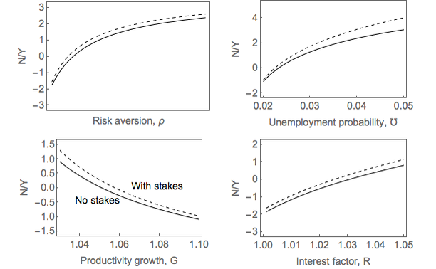
Figure 3 shows the sensitivity of N∕ to changes in ρ, ℧, G and R. The death
probability D was adjusted so as to keep the total expected lifetime of an
individual equal to sixty years, i.e.,
to changes in ρ, ℧, G and R. The death
probability D was adjusted so as to keep the total expected lifetime of an
individual equal to sixty years, i.e.,
First, we observe that the model with stakes gives results that are higher than the model without stakes, but generally provides a good approximation for the variation of the net foreign assets with respect to the main parameters.
The variation with respect to the growth rate and the unemployment probability confirm theoretical properties derived earlier. The foreign assets ratio decreases with G, as predicted by (18). The ratio of foreign assets to GDP also increases with the unemployment probability. The ratio of foreign assets to GDP is increasing with risk aversion ρ. Finally, the foreign asset ratio is increasing with R, mainly because of the impact of higher interest rates in reducing the ratio of physical capital to output. The wealth-to-GDP ratio (not reported in Figure 3) is not very sensitive to R, which is consistent with the ambiguity of the model prediction if ρ > 1.
In this section, we relate our model’s stylized treatment of uncertainty to the treatment in a related model with a much more realistic (but much less tractable) structure. Specifically, we use the model in Carroll, Slacalek, Tokuoka, and White (2017) (henceforth ’CSTW’), which incorporates transitory and permanent idiosyncratic shocks a la Friedman (1957) calibrated to match empirical estimates of the magnitude of such household-level shocks in U.S. data. We use that model to calculate a quantitative relationship between the central measures of uncertainty in the two models, and show how this helps provide an interpretation of the quantitative relationship of uncertainty to precautionary saving in our model.
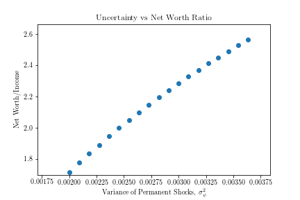
The CSTW model specifies a household income process commonly used in the modern microfounded consumption literature. Household income yt is determined by the aggregate wage rate Wt and two idiosyncratic components, the permanent component pt and the transitory shock ξt:
| yt = ptξtWt | (27) |
| pt = pt−1ψt | (28) |
CSTW find that in order for the model to generate a plausible distribution of wealth it is necessary to build in some form of ex ante hetergogeneity; we follow them in assuming that the time preference rate is the locus of heterogeneity, and in calibrating the mean of the time discount factor to match the U.S. aggregate wealth to income ratio and the the spread of the time discount factor to match the wealth distribution among households in U.S. data.16
Following CSTW, we set the benchmark annual values of σψ2 and σ𝜃2 to be 0.010 and
0.010.17 The
growth impatience condition Þ of the most patient agent restricts the maximum value of σψ2
we can choose.18
of the most patient agent restricts the maximum value of σψ2
we can choose.18
Our unemployment shock is a permanent shock to income, so it is natural to interpret alternative values of ℧ as proxying for differences in the variance of permanent shocks σψ2. The difficulty is in knowing quantitatively how to translate alternative values of ℧ into the corresponding values of σψ2.
To help with the translation we have constructed a rough bridge between the two models, as follows. First, we set the parameters that the two models share, G, Ξ,ρ,R,X, to the same values (the values reported in Table 1). And we set the values of parameters unique to the CSTW model to their default values from that paper.
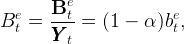
Next, we find a value of ℧ at which the two models predict the same ratio of aggregate wealth to income, B. Here, the tractability of our model comes in handy; although the analytical function for B in terms of primitives19 is not analytically invertible, it is well-behaved (under appropriate parametrica assumptions) so that finding the ℧ for which B matches any particular value is numerically trivial.
For the case in hand, the CSTW model’s value is = 2.56 (matching the target from a 2010 JEDC symposium organized by Den Haan, Judd, and Juillard (2010) on solution methods for models of this class), and we calculate that our model generates B = 2.565 for ℧ ≈ 0.01167 ≡.
The last step is to map deviations of the two variables, ℧ in the tractable model and σψ2 in the CSTW model, from their benchmark values in such a way that, locally, the mapped change in ℧ generates the same change in B as the corresponding change in σψ2.
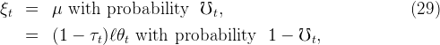
It turns out that the relationships between steady-state net worth and our principal measures of uncertainty are not far from linear in either model; see ?? and ?? for plots of the relation between B and each model’s central measure of uncertainty (℧ for the tractable model; σψ2 for CSTW), over the range from half the benchmark value to the full benchmark value. Because it is computationally expensive to calculate, the results from the CSTW model are presented at a set of points sufficient to reveal the shape of the underlying continuous function; because it is analytic, we can plot the function for the tractable model exactly.
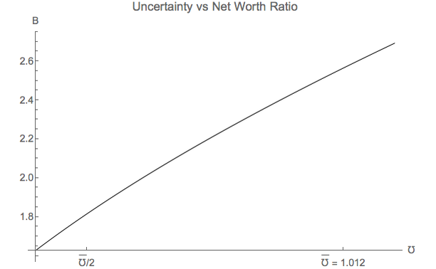
The two figures are encouragingly similar to each other over the corresponding ranges of their chief uncertainty measures, so we are comfortable in approximating the first order relationships in the vicinity of the target by


Under these assumptions, there is some ν such that
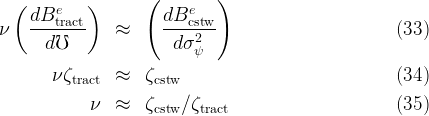
When we undertake this exercise, we obtain a value of ν ≈ 0.254. That is, the conclusion is that a rough interpretation of a one unit change in ℧ is that it is equivalent to a change of about (1∕4) as much in the measurable quantity σψ2.
There is at present little evidence on the size of ζcstw. But recent years have seen a growing number of estimates of statistics like σψ2 across countries. Studies comparing small open economies with well-measured data both on saving rates and proxies for σψ2 should be able to measure an empirical counterpart to ζcstw, if variations in this statistic are in fact large enough to contribute importantly to the difference in saving rates across countries (as, for example, the IMF seems to believe is true [cite IMF advice to China to bolster its social safety net to encourage consumption]).
The Ramsey model corresponds to the particular case where the economy is populated by one representative infinitely-lived worker (Ξ = 1 and ℧ = 0). Thus, one might expect our model to yield the same results as the Ramsey model in the limiting case as population growth and unemployment risk go to zero (Ξ and ℧ → 0).
In fact this is not the case. The predictions of our model for net foreign assets and capital flows exhibit a discontinuity at ℧ = 0. To see this, note that taking the limit of equation (17) gives
 |
so that the ratio of total domestic wealth to GDP goes to zero as the risk of unemployment becomes vanishingly small,20
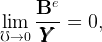 |
implying that the ratio of foreign assets to GDP is equal to minus the ratio of capital to output,
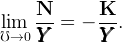 | (36) |
The Ramsey model does not yield the same formula. If the unemployment risk is strictly equal to zero (℧ = 0), we must assume Γ < R for the intertemporal income of the worker to be well-defined and finite.21 In this case income growth is the same at the individual level and at the aggregate level. We can also assume, without loss of generality, that X = 1, so that Γ = G. Then it is possible to show that the asymptotic ratio of total net foreign assets to GDP is given by,
 | (37) |
(see the appendix).
Comparing (36) with (37) shows that the ratio of foreign assets to GDP is smaller in the Ramsey model. In fact, it is much smaller for plausible calibrations of the model. The ratio of gross foreign liabilities to GDP implied by the Ramsey model is close to 70 if R = 1.04 and G = 1.03, and goes to infinity as G converges to R from below. The growth impatience condition, which is necessary for the workers to have a finite target for their wealth to income ratio when they are vulnerable to unemployment, makes the infinitely-lived Ramsey consumer willing to borrow a lot against his future income.
The intuition for the discontinuity is that a consumer with CRRA utility will never allow wealth to fall to zero if there is a possibility of becoming permanently unemployed, because unemployment with zero wealth yields an infinitely negative level of utility (if ρ > 1). This is the reflection, in the international macroeconomic context, of a result long understood in the precautionary saving literature: Perfect foresight solutions are not robust to the introduction of uninsurable noncapital income shocks, even if those shocks occur with low probability.22
The model assumes that the income of an unemployed worker falls to zero. This is a reasonable assumption for a country in which unemployed and retired workers receive no social transfer (i.e., in which there are no unemployment benefits and the retirement system is entirely based on capitalization). However, many countries have such transfers, and it is interesting to see their impact on foreign asset accumulation in our model. We consider now the consequences if the government creates a balanced-budget partial ‘unemployment insurance’ system.
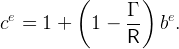
Our definition of partial insurance starts by assuming that the ‘true’ labor income process is the one specified above, but the government interferes with this process by transferring to the workers who become unemployed in period t a multiple ς of the labor income that they would have received if they had remained employed. The social insurance of our model could be interpreted as an unemployment benefit or as a pay-as-you-go retirement benefit.
The wealth of a newly-unemployed worker now includes the payment from the insurance scheme, so that equation (8) becomes:
 |
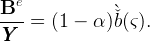
We introduce social insurance in the model with stakes.23 As shown in the appendix, one can compute the target wealth-to-GDP ratio as
where is the asset ratio without insurance, given by (25). The target
wealth-to-income ratio is (linearly) decreasing with ς, as insurance provides a
substitute to precautionary wealth. The formula for N∕
is the asset ratio without insurance, given by (25). The target
wealth-to-income ratio is (linearly) decreasing with ς, as insurance provides a
substitute to precautionary wealth. The formula for N∕ remains (22), with the
ratio of workers’ wealth to GDP given by,
remains (22), with the
ratio of workers’ wealth to GDP given by,
 | (39) |
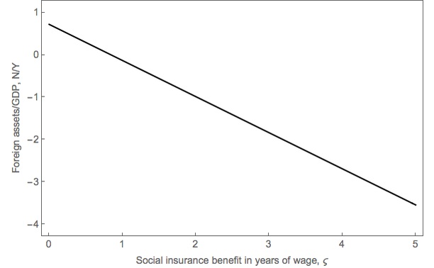
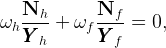
Figure 4 shows how the ratio of foreign assets to GDP, N∕ , varies with ς. The
ratio decreases from 0.72 when there is no insurance to negative values when ς
exceeds 1 year of the worker’s wage. The desired level of foreign assets is thus
quite sensitive to the level of social insurance.
, varies with ς. The
ratio decreases from 0.72 when there is no insurance to negative values when ς
exceeds 1 year of the worker’s wage. The desired level of foreign assets is thus
quite sensitive to the level of social insurance.
Although the model is highly stylized, plausible calibrations can predict ratios of foreign assets to GDP that are close to the levels observed in the real world.24 This section illustrates how our framework can be applied by looking at two questions that have been discussed in recent policy debates and academic research: The relationship between economic development and capital flows, and the long-run consequences of resorbing global imbalances.
Many observers have noted the paradox that international flows of capital have recently been going “upstream” from developing countries (especially in Asia and most notably China) to the United States. The case of China, which has caused so much consternation recently, is merely the latest and largest example of a long-established pattern: Over long time periods and in large samples of developing countries, the countries that grow at a higher rate tend to export more capital (see the evidence cited in footnote 1), a fact that is difficult to reconcile with the standard neoclassical model of growth (Carroll and Weil (1994); Carroll, Overland, and Weil (2000); Gourinchas and Jeanne (2013); Prasad, Rajan, and Subramanian (2007); Sandri (2014)). Can our model shed light on this puzzle?
In this section we look at the correlation between economic growth and capital flows in a given country over time. We assume that the small open economy enjoys an economic “take-off,” defined as a permanent increase in the growth rate of productivity. However, the rate of growth is not the only thing that increases at the time of the transition: Idiosyncratic unemployment risk rises too. An increase in idiosyncratic risk has been observed in many transition countries as they adopt market systems, a development that has not been associated, in most countries, with a corresponding increase in social insurance. In particular, the rise in idiosyncratic risk has been fingered as a reason for the very high saving rate in China (see, e.g., Chamon and Prasad (2010) and the references therein).
Informally, we believe that our story also may relate to the literature on rural-to-urban migration within developing countries. That literature has long struggled to answer a simple question: Urban wages are much higher than rural wages, so why doesn’t everyone move to the city? Maybe the answer is “cities are too risky.” If, in your home village, you are part of a well-developed and robust social insurance network (based on extended family, clan, or village ties), it might be perfectly rational to settle for a low but safe rural standard of living in preference to the more lucrative, but also riskier, life of a city dweller (under the presumption that moving to the city would sever some or all of your ties to the village network, and those ties could not quickly be replaced in a new locale). If people differ in their degree of risk tolerance, the least risk averse will migrate to the cities, leaving the most cautious behind; with a finite population, this could lead to equilibria with large and permanent wage gaps.25
Formally, we assume that the economy starts from a steady state with constant levels for the productivity growth rate and the unemployment probability, Gb and ℧b. At time 0, those variables unexpectedly jump to higher levels, Ga > Gb and ℧a > ℧b. The subscripts b and a respectively stand for “before” and “after” the transition. The death probability is adjusted so as to keep the expected lifetime of an individual equal to 60 years.
Note that in order to benefit the domestic population, the transition must strictly increase the expected present value of an individual’s labor income, given by
 |
Thus one must have,
 | (40) |
The increase in the idiosyncratic risk, in other words, should not be so large relative to the increase in the growth rate as to decrease workers’ expected present value of labor income.
We consider the model with stakes, so that the transition dynamics for aggregate wealth can be derived from those for the representative agent. There is no social insurance. The appendix explains how the path of the main relevant variable can be computed. We are interested in whether capital tends to flow in or out of the country when the transition occurs.
For the sake of the simulation, we assume that the growth rate increases from 2 percent to 6 percent in the transition, whereas the unemployment probability increases from 2 percent to 3 percent (Gb = 1.02, ℧b = 0.02, and Ga = 1.06, ℧a = 0.03). The other parameters remain calibrated as in Table 1.26 Note that condition (40) is satisfied: indeed, the economic transition multiplies the expected present value of individual labor income by a factor 20. If the risk of unemployment did not increase with the transition, the expected net present value of labor income would become infinite.
Figure 7 shows the time paths for the growth rate, the ratio of net foreign assets to GDP and the ratio of capital outflows to GDP, with and without the increase in unemployment risk. Note that if unemployment risk increases, the growth rate takes time to converge to its new higher level because the rate of labor participation decreases over time, which dampens the acceleration of growth. The figure also shows that the increase in idiosyncratic risk has a large impact on the desired level of net foreign assets in the long run—and thus on the direction of capital flows during the transition.
If the level of idiosyncratic risk remains the same, the pickup in growth lowers the long-run level of foreign assets from -23.9 percent to -135.6 percent of GDP, so that the higher growth rate is associated with a larger volume of capital inflows, both in the transition and in the long run. Thus, the model reproduces the usual result from growth models without a precautionary motive: Higher expected growth causes lower saving.
By contrast, if the level of idiosyncratic risk increases along with growth, the long-run level of foreign assets increases to 69.7 percent of GDP, implying that higher growth is associated with capital outflows.27 Thus, small changes in the level of idiosyncratic risk have a first-order impact on the volume and direction of capital flows and may help explain the puzzling correlation between economic growth and capital flows that is found in the data.28
![]()
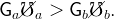
We now look at what the model says about the steady-state correlation between growth and capital flows, rather than the correlation for a given country over time. The country exports capital if its net foreign asset position is positive (N > 0), since the level of its net foreign assets increases over time with output. The ratio of capital outflows to output is given by,
 | (41) |
On the one hand, with faster growth the target value of (N∕ ) will be smaller. On
the other hand, a country that grows faster must export more capital to maintain a
constant ratio of foreign assets to GDP (so the term in parentheses in (41) becomes
larger).29
Even if both initial and final values of (N∕
) will be smaller. On
the other hand, a country that grows faster must export more capital to maintain a
constant ratio of foreign assets to GDP (so the term in parentheses in (41) becomes
larger).29
Even if both initial and final values of (N∕ ) are positive, the sign of the
relation between growth and net capital flows is theoretically ambiguous.
) are positive, the sign of the
relation between growth and net capital flows is theoretically ambiguous.
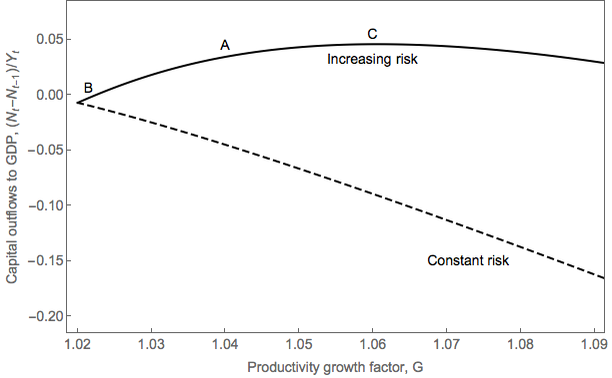
We calibrate the model with the pre-transition regime parameter values (i.e. with G = 1.02 and ℧ = 0.02). Figure 6 shows how the right-hand side of (41) varies with G under two different assumptions. The line “constant risk” shows the ratio of capital outflows to GDP if the only variable that changes is the growth rate. The line “increasing risk” is based on the assumption that the idiosyncratic risk increases linearly by 0.25 percent for every additional percent of growth. Points A, B, and C respectively correspond to the benchmark calibration, the pre-transition regime and the post-transition regime of the previous section.
Two findings stand out. First, if idiosyncratic risk does not increase with growth, the ratio of capital outflows to GDP is decreasing with growth. Second, if idiosyncratic risk increases with growth as we have specified, the ratio of capital outflows to output is positive, i.e., an increase in growth always causes the economy to export more capital (even if it grows at 10 percent per year). The relationship between the ratio of capital outflows to GDP and the growth rate is non-monotonic. Capital outflows increase (as a share of GDP) with the growth rate if the latter is lower than 6 percent. For higher levels of the growth rate the sign of the relationship is reversed.
The main counterpart for the accumulation of net foreign assets by developing countries has been the accumulation of net foreign liabilities by the United States. In a famous 2005 speech, Ben Bernanke hypothesized that the then-prevailing low level of world interest rates and high level of U.S. current account deficits could be due in part to this global “savings glut” (Bernanke (2005)). The U.S. authorities subsequently argued that an orderly resolution of global financial imbalances required the saving rate of Asian emerging market countries, most notably China, to decrease to more normal levels.30
The small economy assumption is not appropriate for studying such large events. We therefore present in this section a two-country general equilibrium version of the model that can be used instead. The model is solved only for the steady state equilibria, which means that we will be interested in the long-term consequences of particular policy experiments. We first look at a closed-economy version of the model.
We assume that the global economy has the same structure as the small open economy that we have considered so far. Global net foreign assets are equal to zero, which using (22) implies
 | (42) |
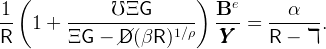
The left-hand side is the desired global stock of wealth whereas the right-hand side is the desired global stock of capital. The equality between the two endogenizes the steady-state interest rate. We assume that the desired stock of wealth comes from the model with stakes and social insurance, i.e., it is given by (39).
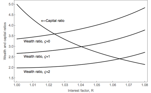
Figure 9 shows how the desired stocks of saving and of capital vary with the interest rate for the benchmark calibration and three different levels of social insurance ς = 0, 1 and 2.31 The desired level of capital is decreasing with the interest rate whereas the desired level of wealth is increasing with the interest rate. Note that the desired level of capital is much more sensitive to the interest rate than the desired level of wealth. This implies that the decrease in desired wealth generated by higher social insurance is reflected almost one for one in a lower level of capital – an interesting point because it illustrates the importance of incorporating the precautionary motive in the model.
This section uses a two-country version of our model to investigate the long-run impact of a decrease in the desired stock of wealth outside of the United States. We consider a two-country world, where each country has the same structure as before. The two countries (denoted by h and f, respectively for “home” and “foreign”) are identical, except for their populations and levels of social insurance (ςh and ςf). The shares of countries h and f in world output are respectively denoted by ωh and ωf. The two countries have the same growth rate, so that there is a well-defined balanced growth path in which each country maintains a constant share of global output.
The condition that global foreign assets must be equal to zero,
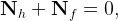 |
endogenizes the global interest rate R. Normalizing by the countries’ GDP, this equation can be rewritten,
 |
where for each country, N∕ is given by (22), with Be∕
 = (1 − α)
 (ς).
(ς).
We consider the following experiment. Assume that the share of the home
country in total GDP is 20 percent (ωh = 0.2 and ωf = 0.8), which is the
right order of magnitude for the United States. Assume that ςh > ςf,
implying that the home country has net liabilities because the desired ratio
of wealth to GDP is lower at home than in the rest of the world. We
assume the values ςh = 1.5 and ςf = 0.75, which implies R = 1.042,
Nh∕ h = −0.512 and Nf∕
 f = 0.128 (the values of the other parameters
remaining as in Table 1). The ratio of U.S. liabilities to GDP is higher than the
current level (which is closer to 25 percent), but not implausible looking
forward if the U.S. were to continue to maintain large current account
deficits.
f = 0.128 (the values of the other parameters
remaining as in Table 1). The ratio of U.S. liabilities to GDP is higher than the
current level (which is closer to 25 percent), but not implausible looking
forward if the U.S. were to continue to maintain large current account
deficits.
We then consider what would happen if global imbalances were resorbed as a consequence of a reduction in the desired wealth-to-income ratio in the rest of the world; this is achieved by increasing ςf to the home level (from 0.75 to 1.5). Figure 8 shows the long-run response of the foreign assets and liabilities, as well as the global real interest rate and real wage (normalized by productivity). As expected, the net foreign assets of the home and foreign countries go to zero as the two countries converge to the same ratio of wealth to GDP. However, this convergence is achieved mainly by a decrease in global capital, which is reflected in an increase in the real interest rate (from 4.2 to 5.6 percent), and a decrease in the normalized real wage (by 5.4 percent).
The decrease in the desired foreign level of wealth thus has a large negative impact on the real wage. The welfare effect is unambiguously negative for the home country. The long-run welfare impact is also negative in the foreign country, although not necessarily during the transition, as the generations that are alive at the time of the increase in social insurance benefit from consuming the accumulated net foreign assets. The home country enjoys an export boom during the transition, but this is associated with lower investment rather than higher output.
The intuition should be clear from the analysis of the closed economy in the previous section. The decrease in the desired level of foreign wealth raises the world interest rate, with little impact on the level of home wealth. Thus, it is reflected mainly in a decrease in the ratio of capital to output, which depresses the real wage.
This paper has presented a tractable model of the net foreign assets of a small open economy. The desired level of domestic wealth was endogenized as the optimal level of precautionary wealth against an idiosyncratic risk. We presented two applications of the model. The first concerned the relationship between economic development and capital flows. The second concerned the long-run global implications of reducing global imbalances by reducing the desired stock of saving outside of the United States.
Although very stylized, the model is able to predict plausible orders of magnitude for the ratio of net foreign assets to GDP. This being said, there are several dimensions in which the model could be made more realistic, at the expense of tractability. In particular, it would be interesting to know the exchange rate implications of a multi-goods extension of the model. (We anticipate that such an extension would show that a developing country that increases its desired level of foreign assets following economic liberalization will see a depreciation of its real exchange rate.) It would be also interesting to look at the impact of changes in the desired level of wealth on the price of assets other than currencies.
Our paper also has potential implications for future empirical work. To the best of our knowledge, the empirical literature has not looked at the impact of idiosyncratic risk and social insurance on net foreign assets in the context of a large sample of countries. The available evidence is anecdotal or focused on one country (e.g., Chamon and Prasad (2010)), or it is about financial development rather than social insurance (Mendoza, Quadrini, and Ríos-Rull (2009)). It would be interesting to see if the predictions of our framework for net foreign assets can be tested with the available data (although we have not been able to find a cross-country database on social insurance that could be used for such an empirical study).
We provide the following tables to aid the reader in keeping track of our notation.
| Parameter | Definition |
| α | Capital’s share in the Cobb-Douglas Production Function |
| ℸ | Depreciation Factor (Proportion Remaining After Depreciation) |
| Ξ | Population Growth Factor |
| G | Aggregate Productivity Growth Factor |
| R | Riskfree Interest Factor |
| β | Time Preference Factor |
| ρ | Coefficient of Relative Risk Aversion |
| ς | Severance Payment (In Years Of Income) Paid At Unemployment |
| X | Individual (eXperience-based) Productivity Growth |
| ωi | Weight (Share) Of Country i in World Income |
| ℧ | Probability Of Employed Worker Becoming Unemployed |
| D | Probability of Death |
| τ | Tax Rate |
| χ | ‘Stake’ In Version Of Model With Stakes |
| ξ | Individual’s Employment Status (1 if Employed; 0 if Not) |
Some combinations of the parameters above are used as convenient shorthand:
| Constant | Definition
| ||
 | ≡ | 1 − ℧ | Period Probability of Employed Worker Remaining Employed |
 | ≡ | 1 −D | Probability of Survival (Not Dying) |
 | ≡ | 1 − τ | Proportion of Income Left After Taxation |
| Λ | ≡ |  | Annual Shrinkage of Old Generations’ Share in L |
| κu | ≡ | 1 − | Marginal Propensity to Consume for Unemployed Consumer |
| Γ | ≡ | GX | Labor Income Growth For Continuing-Employed Individual |
| ÞΓ | ≡ |  | Growth Patience Factor |
| Variable | Definition |
| C | Consumption |
| ℰ | Employed Population |
| I | Investment |
| K | Physical Capital Stock |
| L | Labor Supply |
| ℓ | Individual labor productivity per employed worker |
| N | Net Foreign Assets |
| P | GDP (‘Production’) |
| B | Total Wealth (Foreign and Domestic) |
| 𝒰 | Unemployed Population |
| Typeface | Meaning
|
| Bold | Level of a Variable |
| Plain | Ratio of The Variable To GDP or Labor Income |
| Uppercase | Aggregate Variable |
| Lowercase | Household-Level (Idiosyncratic) Variable |
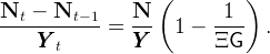
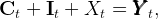
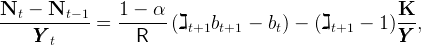
The aggregate budget constraint of residents can be written,
 |
Using (2) this equation can be rewritten as,
 |
where It = Kt+1 − ℸKt is domestic investment, and Nt is given by (5). Using the GDP identity (domestic output is either consumed, invested or exported), and defining X as net exports, we have
 |
it follows that net exports are equal to Xt = Nt −RNt−1. By definition, the current account balance is equal to net exports plus the income on net foreign assets,
 |
from which we can derive the balance-of-payments equation,
 |
The current account balance is equal to the increase in the country’s net foreign asset position, i.e., the volume of capital outflows in period t.
An insurance company a la Blanchard (1985) provides each newly unemployed worker with an annuity, i.e., a consumption path that is conditional on the individual staying alive. The annuity contract maximizes the welfare of the individual conditional on the expected present value of his consumption being equal to his wealth. For a worker becoming unemployed at t it solves the problem,32
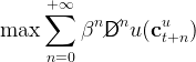 |
subject to
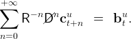
The Euler equation is,
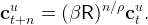 |
Using this expression to substitute out ct+nu from the expected present value constraint then gives,
 |
We first characterize the iso-be and iso-ce loci in the space (be,ce). Equation (13) implies that the iso-be locus is a line defined by,
 |
Similarly, setting cet+1 = cet in equation (14) gives the following equation for the iso-ce locus,
![[ ]
( − ρ ) − 1∕ρ − 1
ce = 1 + -Γ--- 1 + ÞÞÞΓ---−-1-- (1 + be).
κuR ℧](cjSOE109x.png) |
The iso-ce locus is an upward-sloping line which intersects the ce-axis below
the iso-be line. The iso-ce line and the iso-be lines intersect in the positive
quadrant (as indicated on Figure 1) if and only if  > 0. This is true
because,
> 0. This is true
because,
 |
where the last inequality follows from the growth impatience condition (11).
Using equation (13), it is straightforward to see that be increases (decreases) if and only if (be,ce) is below (above) the iso-be line. Equation (14) implies that cet+1 is decreasing with bet. Therefore, ce decreases if and only if (be,ce) is in the region to the right of the iso-ce locus. This is also the region below the locus, because this locus is upward-sloping. Thus, the phase diagram is as it is shown on Figure 1, and the dynamics for the pair (bet,cet) are saddle-point stable.
Here we derive equation (19). The aggregate wealth of employed workers is given by,
 |
where et,t−n is the number of employed workers born in period t − n, and
bet,t−n = bet,t−nWtℓn is the level of wealth held by the representative worker in
the generation born at t − n. Using et,t−n = Ξt−n n and ℓn = Xnℓ0 we
have
n and ℓn = Xnℓ0 we
have
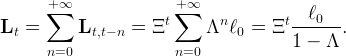
 |
with Λ =  X∕Ξ. Using
  t = WtLt∕(1 − α) the ratio of foreign assets to output
can be written
t = WtLt∕(1 − α) the ratio of foreign assets to output
can be written
 | (43) |
Each individual has a labor endowment that increases at rate X until he becomes unemployed. Thus, in period t the generation born at t − n supplies a quantity of labor equal to the number of workers from this generation who are still employed at t, times the labor supply per worker,

 | (44) |
Using this expression to substitute out Lt from equation (43) then gives equation (19).
We add to the model a transfer that ensures that the workers have the same wealth-to-income ratio at all times. More precisely, the transfer ensures that if all workers have the same ratio be in period t, then this is also true in period t + 1. So one simply needs to assume that all workers had the same ratio be at some point in the past for this to be true in all periods. This would be the case, for example, if the country started with a first generation at some distant period in the past.
The period-t budget constraint of an individual is
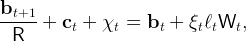 |
where χt is a lump-sum transfer. The transfer puts newborn individuals at the same net wealth-to-income ratio as the rest of the population. For the other workers the transfer is a lump-sum tax that is proportional to their generation’s wealth. For an employed worker born at t − n the tax is,
 | (45) |
whereas for a new-born worker the transfer is given by,
 | (46) |
In all periods of a worker’s life, thus, the normalized budget constraint is given by,
 | (47) |
which generalizes (13). Equation (15) remains valid,
 |
whereas (16) is replaced by
 |
Eliminating  between these two equations then gives the following expression for
the target wealth-to-income ratio,
between these two equations then gives the following expression for
the target wealth-to-income ratio,
![[ ]− 1
( − ρ )1 ∕ρ
ˇˇb = Γ- − /τ + κu 1 + ÞÞÞ-Γ--−--1- .
R ℧](cjSOE127x.png) | (48) |
The equilibrium level of τ results from the following equality,
 |
The left-hand side is the flow of payment that is required to endow each newborn
individual with the same ratio of after-tax net wealth to income as the rest of
the population. The right-hand side is the proceeds of the tax on the
employed workers. Using (44) to substitute out Lt, this equation simplifies to
 = τ∕(1 − Λ), which implies
 | (49) |
Using this expression to substitute out τ from (48) gives (25).
In this model, the economy consists of a continuum of households of mass one
distributed on the unit interval. Households die with a constant probability
D = 1 − between periods. (This is different from our baseline model in which
households only face probability of dying after they become unemployed.) The
income process was described in section 3.2. Each household maximizes expected
discounted utility from consumption:
between periods. (This is different from our baseline model in which
households only face probability of dying after they become unemployed.) The
income process was described in section 3.2. Each household maximizes expected
discounted utility from consumption:
 | (50) |
The household consumption function c satisfies:
where the variables are divided by the level of permanent income = pt
= pt , so
that when aggregate shocks are shut down, the only state variable is
(normalized) cash-on hand mt. The production function is Cobb-Douglas:
, so
that when aggregate shocks are shut down, the only state variable is
(normalized) cash-on hand mt. The production function is Cobb-Douglas:
| ZKα(ℓL)1−α | (51) |
 t is determined by the aggregate productivity Zt,
capital stock Kt, and the aggregate supply of labor Lt:
t is determined by the aggregate productivity Zt,
capital stock Kt, and the aggregate supply of labor Lt:
 t = (1 − α)Zt( t = (1 − α)Zt( )α )α | (52) |
| Lt = PtΘt | (53) | |
| Pt = Pt−1Ψt | (54) |
The Ramsey model corresponds to the particular case where there is one representative infinitely-lived worker (Ξ = 1 and ℧ = 0). In this case income growth is the same at the individual level and at the aggregate level. We can assume, without loss of generality, that X = 1, so that Γ = G.
The individual’s problem at time 0 is to maximize,
 |
subject to the budget constraint,
 |
where  t = Gt
 0 is the country’s output. For the worker’s discounted
intertemporal income to be finite we must assume G < R.
0 is the country’s output. For the worker’s discounted
intertemporal income to be finite we must assume G < R.
Iterating on the budget constraint and using ct = (βR)t∕ρc0 (from the Euler
equation) and  t = Gt
 0 to substitute out consumption and output, we have
 |
The limiting wealth-to-output ratio is given by,
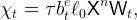
Here we derive equation (38). The worker’s normalized budget constraint is still given by (47), taking into account that the wage is taxed at rate τw to pay for the unemployment benefits,
 | (55) |
Equation (12) still applies, with cut+1 = κu(bet+1 + ς). Setting bet+1 = bet =  and cet+1 = cet =
  in equations (12) and (55) we obtain
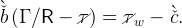
 between these equations gives,
![[ ( ) ]
ÞÞÞ − ρ − 1 1∕ρ
`ˇb = /τw − κu 1 + --Γ------- ς ˇˇb,
℧](cjSOE154x.png) | (56) |
where  is given by equation (25). The tax rate τw must satisfy
 | (57) |
The left-hand-side is the flow of tax receipts at time t. The right-hand-side is the amount needed to finance the transfer to the newly unemployed workers. Using ℓt = Lt∕ℰt and ℰt∕ℰt−1 = Ξ one has,
 |
Using this expression and (49) to substitute out τw from equation (56) gives equation (38).
Normalizing ℓ0 to 1, the equation for the dynamics of aggregate labor supply is,
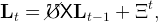 |
implying that in steady state,
 |
Up until period 0 (inclusive), the economy is in a steady growth path with G = Gb and ℧ = ℧b, so that
 |
In period 0 it is announced that from period 1 onwards the productivity growth rate and the flow probability of unemployment jump to higher levels, Ga and ℧a. Starting from L0, the dynamics of labor supply are given by,
 |
from which it is possible to compute the whole path (Lt)t≤0, as well as the gross
rate of growth in labor supply, Lt∕Lt−1. It follows from (1) and (2) that output
grows at the same rate as ztLt. Hence the gross rate of output growth,
ℷt ≡ t∕
t∕ t−1, is given by
 |
for t ≥ 1. Using this expression we can compute the whole path (ℷt)t≥1.
We now come to the ratios of net foreign assets and capital outflows to GDP,
Nt∕ t and (Nt −Nt−1)∕
 t. Using the definition of N equation (5), we
have
t. Using the definition of N equation (5), we
have
![[ ]
N (1 − α )b K
--t-= ℷt+1 ---------t+1-− --- ,
YYY t R YYY](cjSOE167x.png) |
 |
where bt = bet + but is the ratio of aggregate wealth to aggregate labor income. The path for bet is the individual convergence path for the model with stakes, where the initial condition be0 is given by (25) with G = Gb and ℧ = ℧b. This gives us the whole path (bet)t≤0. As for but, the initial condition can be derived from equation (21),
 |
The path for but can then be derived from equation (20), which can be rewritten in normalized form,
 |
Here we describe our algorithm for finding the consumption function.
We know two points on the “true” consumption function: For wealth of
zero, consumption must be zero; and for wealth equal to its target value,
consumption must equal its target value. We can thus construct a crude starting
approximation to the consumption function as 0ce(be) = (č∕ )be, the unique line
that goes through the points {0., 0.} and {
)be, the unique line
that goes through the points {0., 0.} and { ,č} (where the 0 presubscript
indicates that we have executed zero iterations of the ‘improvement’ algorithm
described below).
,č} (where the 0 presubscript
indicates that we have executed zero iterations of the ‘improvement’ algorithm
described below).
We will need to improve upon this approximation considerably in order to
obtain a satisfactory solution to the model. Our first step is to construct a set of
points at which to evaluate any approximating function, which we choose on the
interval [0, 2 ]. Dividing that interval equally into n subintervals, we obtain a set
of states b[i] = 2
]. Dividing that interval equally into n subintervals, we obtain a set
of states b[i] = 2 (i∕n) for i = 0, 1,...,n.
Now rewrite the Euler equation (12) as
 |
and note that starting with iteration m = 0 we can generate a ‘next’ set of consumption points from the current points using
![( )
ce[i] = 1---//℧ ( ce ((R∕ Γ ) (be[i] − ce[i] + 1))− ρ + ℧ (κu (R∕ Γ ) (be[i] − ce[i] + 1 ))− ρ − 1∕ρ
m+1 ÞÞÞΓ m m m](cjSOE176x.png) | (58) |
We solve by using iteration. The iterative scheme stops when successive approximate consumption functions change little at grids.
Given the initial function for m = 0, 0ce(b), the algorithm can be summarized as follows:

For use below, note that we can invert (??) to express the parameters as an implicit function of target of target wealth:
![( ) [ ( − ρ )1 ∕ρ]
1-−--α- Γ- ---1--- u ÞÞÞ-Γ--−--1-
ˇˇ = R − 2 − Λ + κ 1 + ℧ (59 )
B
{ ( ) } [( − ρ )1 ∕ρ]
1-−--α- Γ- ---1--- ÞÞÞ-Γ--−--1-
ˇˇ − R + 2 − Λ = 1 + ℧ (60 )
B
{ ( ) } ρ ( − ρ )
1-−--α- − Γ-+ ---1--- = 1 + ÞÞÞ-Γ--−--1- (61 )
Bˇˇ R 2 − Λ ℧
{ ( ) } ρ − ρ
1-−-α-- Γ- ---1--- ÞÞÞ-Γ--−--1-
ˇ − + − 1 = (62 )
[{ ( ˇB) R 2 −} Λ ] ℧
1 − α Γ 1 ρ − ρ
------- − -- + ------- − 1 ℧ = ÞÞÞ Γ − 1 (63 )
ˇˇB R 2 − Λ
[{ ( ) } ρ ]− 1 ( )
℧ = 1-−-α-- − Γ-+ ---1--- − 1 ÞÞÞ − ρ −(614 )
ˇˇ R 2 − Λ Γ
B](cjSOE178x.png)
Aguiar, M., and M. Amador (2011): “Growth in the Shadow of Expropriation,” The Quarterly Journal of Economics, 126(2), 651–697.
Angeletos, George-Marios, and Vasia Panousi (2011): “Financial Integration, Entrepreneurial Risk and Global Dynamics,” Journal of Economic Theory, 146(3), 863–896.
Arbatli, Elif C. (2008): “Persistence Of Income Shocks And The Intertemporal Model Of The Current Account,” Ph.D. thesis, Johns Hopkins University.
Attanasio, Orazio, Lucio Picci, and Antonello Scorcu (2000): “Saving, Growth, and Investment: A Macroeconomic Analysis Using a Panel of Countries,” Review of Economics and Statistics, 82(1).
Bacchetta, Philippe, and Kenza Benhima (2015): “The Demand for Liquid Assets, Corporate Saving and Global Imbalances,” Journal of the European Economic Association, forthcoming.
Barro, Robert J. (2006): “Rare Disasters and Asset Markets in the Twentieth Century,” Quarterly Journal of Economics, 121(3), 823–66.
Benhima, Kenza (2013): “A Reappraisal of the Allocation Puzzle through the Portfolio Approach,” Journal of international Economics, 89(2), 331–346.
Bernanke, Ben (2005): “The Global Saving Glut and the U.S. Current Account Deficit,” Remarks at the Sandridge Lecture, Virginia Association of Economics, Richmond, Virginia, March 10, 2005.
Blanchard, Olivier J. (1985): “Debt, Deficits, and Finite Horizons,” Journal of Political Economy, 93(2), 223–247.
Buera, Francisco, and Yongseok Shin (2009): “Productivity Growth and Capital Flows: The Dynamics of Reform,” NBER Working Paper 15268.
Caballero, Ricardo J., Emmanuel Farhi, and Pierre-Olivier Gourinchas (2008): “An Equilibrium Model of "Global Imbalances" and Low Interest Rates,” American Economic Review, 98(1), 358–388.
Carroll, Christopher D. (2000): “‘Risky Habits’ and the Marginal Propsensity to Consume Out of Permanent Income,” International Economic Journal, 14(4), 1–41, http://econ.jhu.edu/people/ccarroll/riskyhabits.pdf.
__________ (2016a): “Lecture Notes: A Tractable Model of Buffer Stock Saving,” Discussion paper, Johns Hopkins University, At http://econ.jhu.edu/people/ccarroll/public/lecturenotes/consumption.
__________ (2016b): “Theoretical Foundations of Buffer Stock Saving,” manuscript, Department of Economics, Johns Hopkins University, Available at http://econ.jhu.edu/people/ccarroll/papers/BufferStockTheory.
Carroll, Christopher D., Jody R. Overland, and David N. Weil (2000): “Saving and Growth with Habit Formation,” American Economic Review, 90(3), 341–355, http://econ.jhu.edu/people/ccarroll/AERHabits.pdf.
Carroll, Christopher D., Jiri Slacalek, Kiichi Tokuoka, and Matthew N. White (2017): “The Distribution of Wealth and the Marginal Propensity to Consume,” Quantitative Economics, 8, 977–1020, At http://econ.jhu.edu/people/ccarroll/papers/cstwMPC.
Carroll, Christopher D., and Patrick Toche (2009): “A Tractable Model of Buffer Stock Saving,” NBER Working Paper Number 15265, http://econ.jhu.edu/people/ccarroll/papers/ctDiscrete.
Carroll, Christopher D., and David N. Weil (1994): “Saving and Growth: A Reinterpretation,” Carnegie-Rochester Conference Series on Public Policy, 40, 133–192, http://econ.jhu.edu/people/ccarroll/CarrollWeilSavingAndGrowth.pdf.
Chamon, Marcos, Kai Liu, and Eswar S. Prasad (2010): “Income Uncertainty and Household Savings in China,” Discussion paper, National Bureau of Economic Research.
Chamon, Marcus D., and Eswar S. Prasad (2010): “Why Are Saving Rates of Urban Households in China Rising?,” American Economic Journal: Macroeconomics, 2(1), 93–130, Available at http://www.aeaweb.org/articles.php?doi=10.1257/mac.2.1.93.
Coeurdacier, Nicolas, Stéphane Guibaud, and Keyu Jin (2015): “Credit Constraints and growth in a Global Economy,” American Economic Review, 105(9), 2838–81.
Den Haan, Wouter J, Kenneth L Judd, and Michel Juillard (2010): “Computational suite of models with heterogeneous agents: Incomplete markets and aggregate uncertainty,” Journal of Economic Dynamics and Control, 34(1), 1–3.
Durdu, Ceyhun Bora, Enrique G. Mendoza, and Marco E. Terrones (2009): “Precautionary Demand for Foreign Assets in Sudden Stop Economies: an Assessment of the New Mercantilism,” Journal of Development Economics, 89, 194 – 209.
Fogli, Alessandra, and Fabrizio Perri (2006): “The ‘Great Moderation’ and the U.S. External Imbalance,” NBER Working Paper Number w12708.
Friedman, Milton A. (1957): A Theory of the Consumption Function. Princeton University Press.
Ghosh, Atish R., and Jonathan D. Ostry (1997): “Macroeconomic Uncertainty, Precautionary Saving, and the Current Account,” Journal of Monetary Economics, 40, 121–139.
Gourinchas, Pierre-Olivier, and Olivier Jeanne (2013): “Capital Flows to Developing Countries: The Allocation Puzzle,” Review of Economic Studies, 80, 1484–1515.
Hausmann, Ricardo, Lant Pritchett, and Dani Rodrik (2005): “Growth Accelerations,” Journal of Economic Growth, 10(4), 303–329.
Jeanne, Olivier (2007): “International Reserves in Emerging Market Countries: Too Much of a Good Thing?,” Brookings Papers on Economic Activity, 2007, 1–55.
Jeanne, Olivier, and Romain Rancière (2011): “The Optimal Level of Reserves for Emerging Market Countries: Formulas and Applications,” Economic Journal, 121(555), 905–930.
Kimball, Miles S. (1990): “Precautionary Saving in the Small and in the Large,” Econometrica, 58, 53–73.
Lane, Philip R., and Gian Maria Milesi-Ferretti (2007): “The External Wealth of Nations Mark II: Revised and Extended Estimates of Foreign Assets and Liabilities,” Journal of International Economics, 73(2), 223–250.
Loayza, Norman, Klaus Schmidt-Hebbel, and Luis Servén (2000): “What Drives Saving Across the World?,” Review of Economics and Statistics, 82(1).
Mankiw, N. Gregory (1995): “The Growth of Nations,” Brookings Papers on Economic Activity, 1995(1), 275–326.
Mendoza, Enrique G., Vincenzo Quadrini, and José-Víctor Ríos-Rull (2009): “Financial Integration, Financial Development, and Global Imbalances,” Journal of Political Economy, 117(3).
Merton, Robert C. (1969): “Lifetime Portfolio Selection under Uncertainty: The Continuous Time Case,” Review of Economics and Statistics, 50, 247–257.
Munshi, Kaivan, and Mark Rosenzweig (2009): “Why is Mobility in India so Low? Social Insurance, Inequality, and Growth,” Working Paper 14850, National Bureau of Economic Research.
Obstfeld, Maurice, and Kenneth Rogoff (1995): “The Intertemporal Approach to the Current Account,” in Handbook of International Economics, ed. by Gene M. Grossman and Kenneth Rogoff (North Holland, Amsterdam), 3, 121–139.
Prasad, Eswar, Raghuram Rajan, and Arvind Subramanian (2007): “Foreign Capital and Economic Growth,” Brookings Papers on Economic Activity, pp. 153–230.
Rietz, Thomas A. (1988): “The Equity Risk Premium: A Solution,” Journal of Monetary Economics, 22(1), 117–131.
Samuelson, Paul A. (1969): “Lifetime Portfolio Selection by Dynamic Stochastic Programming,” Review of Economics and Statistics, 51, 239–46.
Sandri, Damiano (2014): “Growth and Capital Flows with Risky Entrepreneuship,” American Economic Journal: Macroeconomics, 6(3), 102–23, http://llorracc.net/Papers/sandriGrowth.pdf.
Song, Zheng, Kjetil Storesletten, and Fabrizio Zilibotti (2011): “Growing Like China,” The American Economic Review, 101(1), 196–233.
Song, Zheng Michael, and Dennis Tao Yang (2010): “Life Cycle Earnings and Saving in a Fast-Growing Economy,” Manuscript, Chinese University of Hong Kong.
Toche, Patrick (2005): “A Tractable Model of Precautionary Saving in Continuous Time,” Economics Letters, 87(2), 267–272, http://ideas.repec.org/a/eee/ecolet/v87y2005i2p267-272.html.
Townsend, Robert (1994): “Risk and Insurance in Village India,” Econometrica, 62(3), 171–84.
Wen, Yi (2009): “Saving and Growth Under Borrowing Constraints: Explaining the ’High Saving Rate’Puzzle,” FRB of St. Louis Working Paper No 2009-45.
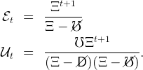
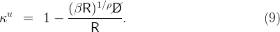
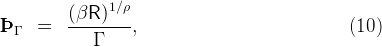

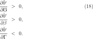
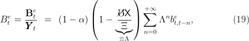
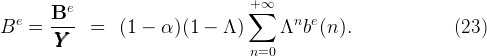
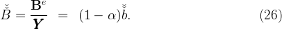
![{ [ ( )1 ∕ρ]}
` ℧ ÞÞÞ − ρ− 1 ˇ
ˇb(ς) = 1 − ς -- + κu 1 + --Γ------- ˇb, (38)
Ξ ℧](cjSOE73x.png)