The American Consumer:
Reforming, Or Just Resting?
June 20, 2009
Christopher D. Carroll1
Johns Hopkins University
Jiri Slacalek2
European Central Bank
_____________________________________________________________________________________
Abstract
American households have received a triple dose of bad news since the beginning of the current
recession: The greatest collapse in asset values since the Great Depression, a sharp tightening in credit
availability, and a large increase in unemployment risk. We present measures of the size of these
shocks and discuss what a benchmark theory says about their immediate and ultimate consequences.
We then provide a forecast based on a simple empirical model that captures the effects of wealth
shocks and unemployment fears. Our short-term forecast calls for somewhat weaker spending, and
somewhat higher saving rates, than the Consensus survey of macroeconomic forecasters. Over
the longer term, our best guess is that the personal saving rate will eventually approach
the levels that preceded period of financial liberalization that began in the late 1970s.
-
Keywords
-
Consumption/Saving Forecast, Credit Crunch, Financial
Crisis
-
JEL codes
-
C61, D11, E24
1Carroll: ccarroll@jhu.edu, Department of Economics, Johns Hopkins University, Baltimore
Maryland 21218, USA; and National Bureau of Economic Research.
2Slacalek: jiri.slacalek@ecb.int, Monetary Policy Research Division, European Central Bank,
Frankfurt Germany. The views contained in this paper do not necessarily reflect the views of the
European Central Bank or other members of its staff.
1 Introduction
Economists and pundits have complained for years that Americans do not save
enough. Economists, in keeping with our reputation, have tended to use bland
words like “unsustainable” or “problematic”; pundits, preferring more
colorful language, have called the American saving rate “dismal” and
“pathetic.”
As economists, we lean toward the bland terminology. But, to quote former
Council of Economic Advisors chair Herbert Stein, “Unsustainable trends, sooner
or later, come to an end.”
That end appears now to be coming, much more suddenly than anyone
expected. Indeed, the collapse in household spending over the past six months is
a principal source of the gloom currently emanating from macroeconomic
forecasters.
After so much lamentation about low saving, it may be a bit hard for the
public to stomach economists’ new worries about a drop in spending. But the
contradiction can be understood by analogy to the prayer of Saint Augustine,
who after a youth spent in debauchery decided to convert to Christianity to
preserve his mortal soul. He was still enjoying his sinful ways when he made that
fateful decision, so his first prayer was “Lord, make me chaste – but not quite
yet.”
Saint Augustine may not have had a good excuse for gradualism, but
economists do: The costs of adjustment to a permanently higher saving rate
would likely be substantially smaller if that increase were spread out over the
course of several years than if it happens all at once. (This is part of the
motivation behind several items in the recently passed stimulus bill that aimed
to revive near-term consumer spending, especially on durable goods like
automobiles.)
Optimal or not, our best guess (illustrated below by forecasts from a simple
model) is that the drop in overall consumption spending will not be speedily
reversed; indeed, we project that the saving rate will rise a bit further from
current levels before stabilizing somewhere not far below the saving rates that
prevailed before the era of financial liberalization that started in the late 1970s.
But we would not be greatly surprised if the saving rate ultimately rises even
more than in our most extreme projection. In answer to the question in our title,
our view is that American consumers are not merely resting from their
former role as the world’s champion consumers, they are permanently
reforming their spending patterns, in response to the end of the period of
ever-more-available credit that fueled the unsustainably high spending of recent
years.
2 Theory and Data
2.1 A Simple Model
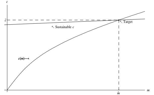
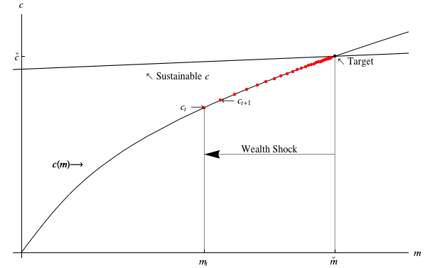
Figure 1 depicts a consumption function  that relates a stylized consumer’s
optimal spending-to-labor-income ratio
that relates a stylized consumer’s
optimal spending-to-labor-income ratio  to the monetary-resources-to-labor-income
ratio
to the monetary-resources-to-labor-income
ratio  ; the consumer is assumed to be behaving according to a simple
buffer-stock saving model like that of Carroll (2009). This consumer is
impatient: In the absence of uncertainty, spending would exceed the amount
consistent with wealth maintenance. For such a consumer, precautionary motives
are the only reason to hold any positive wealth. (The consumption function is
concave because at lower and lower levels of wealth the consumer’s precautionary
motive gets stronger and stronger).
; the consumer is assumed to be behaving according to a simple
buffer-stock saving model like that of Carroll (2009). This consumer is
impatient: In the absence of uncertainty, spending would exceed the amount
consistent with wealth maintenance. For such a consumer, precautionary motives
are the only reason to hold any positive wealth. (The consumption function is
concave because at lower and lower levels of wealth the consumer’s precautionary
motive gets stronger and stronger).
The shallowly sloped line plots, for each level of wealth, the level of spending
that is “sustainable” in the sense that, at that level of spending, expected  in the next period will be unchanged from the current level of
  . (Sustainable
spending is simply the sum of expected labor income and expected interest
income; it is upward sloping because with more assets, the consumer expects to
earn more interest income).
. (Sustainable
spending is simply the sum of expected labor income and expected interest
income; it is upward sloping because with more assets, the consumer expects to
earn more interest income).
The target  is the level of
  at which the consumer will choose the
sustainable level of consumption.
at which the consumer will choose the
sustainable level of consumption.
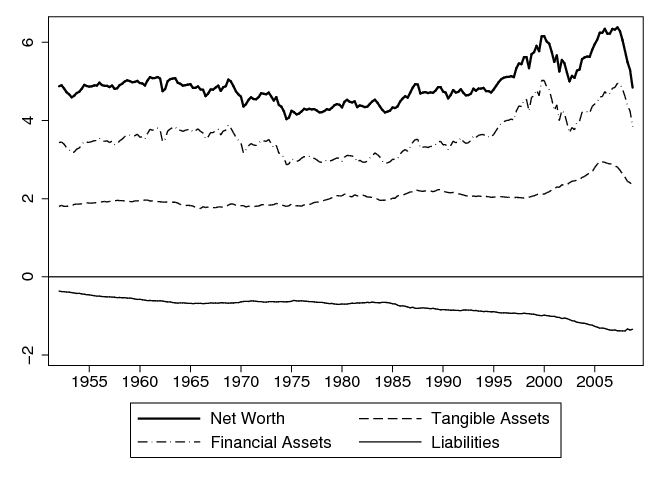
2.2 A Wealth Shock
Our first experiment with the model is motivated by the historic shock to
household wealth depicted in figure 2. Estimates of the magnitude of the wealth
shock range as high as $13 trillion (Baily, Lund, and Atkins (2009)); this is
certainly the largest collapse in asset values since the Great Depression.
Leading up to the period  when the wealth shock occurs, our consumer is
assumed to have been holding the target amount of wealth
when the wealth shock occurs, our consumer is
assumed to have been holding the target amount of wealth  ; the consumer’s
pre-shock position is indicated by the black dot at the point
; the consumer’s
pre-shock position is indicated by the black dot at the point  . In period
 , wealth drops to
  , inducing a corresponding drop in consumption to
  ,
indicated by the red dot at
,
indicated by the red dot at  . The subsequent evolution of consumption
and wealth are represented by the series of red dots leading back toward
. The subsequent evolution of consumption
and wealth are represented by the series of red dots leading back toward
 .
.
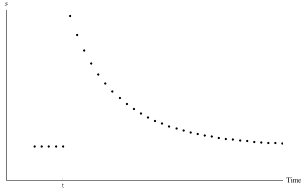
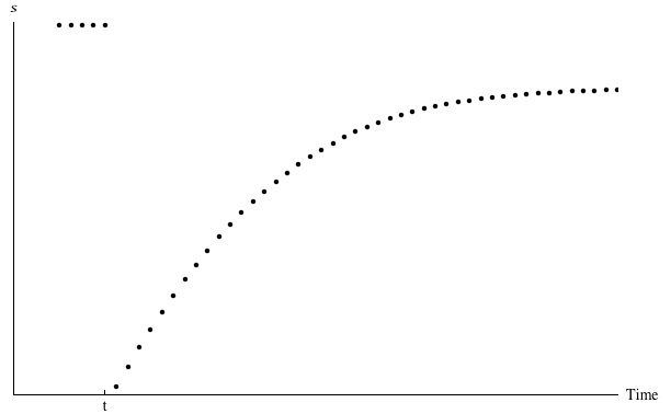
The next figure shows the path of the consumer’s saving rate. Before
the shock, saving was constant at the level necessary to maintain the
wealth-to-income ratio at its target. When the wealth shock hits, the saving rate
jumps up substantially (this is the ‘wealth effect’ in this model). Subsequently, as
wealth builds back up toward its target, the saving rate subsides toward its
equilibrium value.
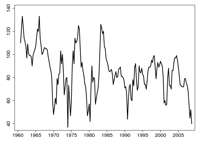
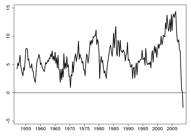
2.3 A Rise In Unemployment Expectations
Figure 5 shows the history of our favorite measure of consumer sentiment: The
University of Michigan’s index of unemployment expectations. In prior work,
we have found that this indicator has substantial predictive power for
consumption spending. And, as the figure shows, the recent survey results show
consumers exhibiting near-record pessimism about future job market
conditions.
Our next experiment, in figure 6, examines the consequences of an increase in
unemployment expectations in the model.
Beginning from the same original consumption function as before,
the new consumption function corresponding to the state of heightened
fear is labelled “ after unemployment rate increase.” Starting,
again, from the original steady state, consumption drops sharply, then as
precautionary wealth builds up spending gradually recovers. The saving path
follows the same pattern as in figure 4: A sudden rise followed by a
gradual subsidence. (The pattern of consumption after the shock is again
indicated by dots. We show only 5 periods of evolution because presumably
unemployment expectations will not remain elevated longer than five years;
when unemployment expectations return to normal, consumption would
jump back to the original consumption function. Of course, real-world
changes in expectations are not likely to be one-off events like those we
simulate, so the changes in spending would not be expected to be so
sharp).
after unemployment rate increase.” Starting,
again, from the original steady state, consumption drops sharply, then as
precautionary wealth builds up spending gradually recovers. The saving path
follows the same pattern as in figure 4: A sudden rise followed by a
gradual subsidence. (The pattern of consumption after the shock is again
indicated by dots. We show only 5 periods of evolution because presumably
unemployment expectations will not remain elevated longer than five years;
when unemployment expectations return to normal, consumption would
jump back to the original consumption function. Of course, real-world
changes in expectations are not likely to be one-off events like those we
simulate, so the changes in spending would not be expected to be so
sharp).
While unemployment expectations will likely return to more normal levels
within a few years, it is possible that the crisis will have a long-lasting
residual effect on consumers’ generalized degree of uncertainty. After the
“Great Moderation” period of relative macroeconomic stability of the
prior twenty years, households’ perceptions of the degree of economic
risk that they were subject to may have fallen substantially. Lingering
memories of the current crisis could therefore have a very long-lasting
effect in boosting the saving rate (and reducing consumers’ appetite for
borrowing).
This leads us to a discussion of the final element of the crisis: Developments in
the credit market.
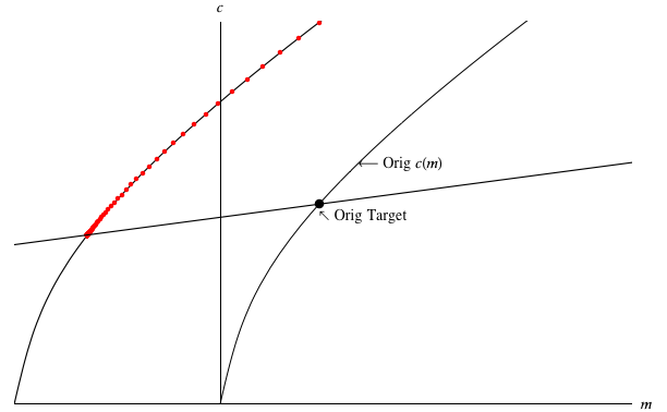
2.4 A Relaxation of Borrowing Constraints
Our final experiment with the model is motivated by the literature that
attributes the runup in consumer debt depicted as the bottom line in figure 2 to
a relaxation of borrowing constraints. The rapid pace of credit expansion,
especially over the past few years, is evident in figure 7. Since the borrowing
outcome depends on both credit demand and credit supply, the rapid pace of
debt growth over this period is not prima facie proof of relaxing credit
conditions; but plenty of evidence suggests that increasing credit availability was
the main driver of credit growth (cf., for example, Mian and Sufi (2008) and the
references therein; see also Dynan and Kohn (2007), who argue that
the increase in house prices was partly responsible for the relaxation of
credit).
The function labelled “Orig  ” in figure 8 reflects an assumed initial
situation in which borrowing is prohibited. The function “New
” in figure 8 reflects an assumed initial
situation in which borrowing is prohibited. The function “New  ” shows
how the consumption function changes if a financial liberalization suddenly
makes borrowing easier. The effect is intuitive: For any given level of monetary
assets
” shows
how the consumption function changes if a financial liberalization suddenly
makes borrowing easier. The effect is intuitive: For any given level of monetary
assets  , the consumer with greater access to credit spends more. Rather than
needing to rely on personal saving as a buffer against uncertainty, the consumer
plans to use his credit line in case of emergencies, so there is less need for direct
wealth holding.
, the consumer with greater access to credit spends more. Rather than
needing to rely on personal saving as a buffer against uncertainty, the consumer
plans to use his credit line in case of emergencies, so there is less need for direct
wealth holding.
Before the relaxation of borrowing constraints, we assume that the
consumer was at the target level of  , as signalized by the black dot at the
intersection of the ‘sustainable
, as signalized by the black dot at the
intersection of the ‘sustainable  ’ line and the consumption function. The
rightmost (highest) red dot on the “New
’ line and the consumption function. The
rightmost (highest) red dot on the “New  ” function shows the
point to which consumption jumps when easier borrowing is allowed; the
remaining dots on the new consumption function show the path by which
consumption evolves downward as wealth falls toward its new, lower
target.
” function shows the
point to which consumption jumps when easier borrowing is allowed; the
remaining dots on the new consumption function show the path by which
consumption evolves downward as wealth falls toward its new, lower
target.
The consumer in our example is so impatient, and the availability of credit
(post liberalization) is so generous, that the new target level of wealth is
negative; in the new equilibrium, the consumer relies upon his borrowing ability
to provide the buffering capacity that was previously provided by his wealth
stock.
The path of the saving rate following the liberalization is shown in figure 9.
The initial upward leap in spending corresponds to a sharp decline in the saving
rate. Subsequently, the saving rate gradually increases, but never fully recovers
to its pre-liberalization level (the lower level of target wealth permitted by
increased borrowing does not require as high a saving rate in order to be
sustained).
This figure underpins our interpretation of the effects of the credit boom of the
past few decades. We view that history as an ongoing sequence of modest
relaxations of borrowing constraints, rather than a giant one-time event. Every
year, credit conditions got slightly easier (with only a few backward
steps). Each particular increase in credit availability would, by itself,
have resulted in a saving response like the one implicit in our figure
(sharp decline followed by gradual recovery); but in each case borrowing
constraints were subsequently further relaxed before the saving rate could
recover. Since credit availability cannot get easier forever (that would be
unsustainable!), the saving rate should stop being depressed whenever
credit-easing ends.
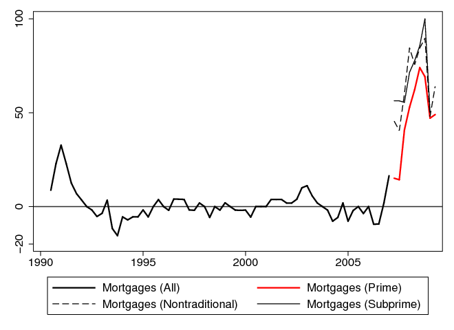
The period of ever-looser credit has certainly now come to an end. Perhaps the
best way to measure changes in the supply of credit is through the Federal
Reserve’s ongoing Senior Loan Officer Opinion Survey, which reports the fraction
of loan officers who say conditions are tightening minus the proportion who say
they are easing. (This only measures conditions at banks, and since much of the
increase in credit supply in the last decade came from nonbank lenders, the
survey is an imperfect measure).
Figure 10, which shows the results of that survey, should remove any doubt
that in the period since the crisis began, credit conditions have tightened
sharply.
The effects of a credit cutback, in the model, are simply the inverse of the
effects of an expansion: Consumption drops, the saving rate rises, and there is
gradual adjustment toward a new equilibrium in which even impatient
consumers find it prudent to hold a larger buffer stock of wealth than
before.
Everyone agrees that much of the credit tightening is necessary and permanent
(the days of No Income, No Job, No Assets (NINJA) mortgage loans will
not return). But the demand for credit has surely fallen also, as fearful
consumers refrain from borrowing even when credit is available to them. Some
combination of reduced demand and tightening supply accounts for the
impressive collapse in net borrowing (‘deleveraging’) shown at the end of
figure 7.
A key question for the longer-term outlook is how long this period of
deleveraging will last, and how much lower the ‘target’ level of leverage is than
its current (still-elevated) level. These are difficult questions with no clear
answer; but we are in the camp that believes that the long-run equilibrium level
of household debt will be substantially lower than the levels of the past few
years, as a result both of consumers’ newfound fears of overindebtedness and as a
result of financial markets’ presumably greater prudence in offering credit going
forward.
3 Consumption So Far
Wealth has cratered; credit availability has tightened sharply; and consumer
confidence has collapsed.
The effect of these events on household spending is best measured using the
BEA’s index of retail sales, which is more timely and less subject to
revision than more comprehensive measures of spending like Personal
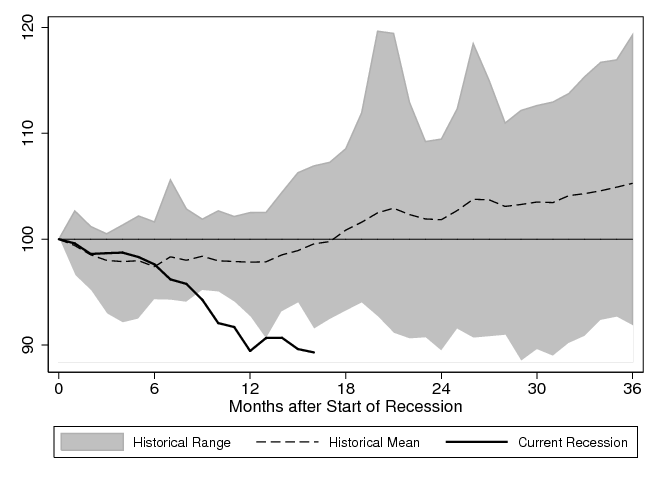
Consumption Expenditures (PCE). Figure 11 shows the level of retail
sales over the period since the beginning of the recession (in December
2007, according to the National Bureau of Economic Research), along
with the pattern of retail sales spending following the other business
cycle peaks in the postwar period. (The level of sales is indexed to 100
at the beginning of each business cycle peak). The gray interval in the
diagram shows, for each month after the recession peak, the minimum
and maximum levels of relative retail sales across all previous postwar
recessions.
Given the magnitude of the shocks, it is no surprise that the figure shows that
the decline in retail sales in the current recession is considerably larger than in
any previous postwar recession. In the latest data available at this writing,
retail sales in April 2009 were estimated to be about 10 percent lower
than when the recession began. In contrast, by this time after previous
recessions peaks, retail sales had on average fully recovered to their peak
level.
Other indicators yield similar conclusions; for example, the decline in
consumption spending in the fourth quarter of 2008 was the sharpest
drop in the past 50 years; a Rockefeller Institute report by Boyd and
Dadayan (2009) finds that state-level data for sales taxes (presumably, an
indicator of sales) showed the sharpest drop in 50 years in the fourth quarter of
2008. Automobile sales have dropped by around 50 percent. And so
on.
4 Our Forecast
The path of consumer spending is famously difficult to forecast. Conveniently,
Robert Hall (1978) provided economists with a good excuse for our forecasting
failures by proving that standard consumption theory implies that forecasting
changes in consumption should be mathematically impossible.
A subsequent literature has nevertheless found some reasonably predictable
patterns in consumption growth. For example, Carroll, Sommer, and
Slacalek (2008) (henceforth, CSS) find that, across a set of 13 developed
economies for which sufficient time series data are available, behavior deviates
from the random walk theory in a simple way: After correcting for measurement
error, consumption growth has a substantial degree of serial correlation, or
‘momentum.’
Concretely, CSS estimate an equation of the form
where the expectation of lagged consumption growth is constructed using data
available at date  (the lag is necessary to correct for measurement
error and time aggregation in the consumption data). At a quarterly
frequency, the serial correlation coefficient for the predictable component of
consumption growth in most countries (including the U.S.) is about
(the lag is necessary to correct for measurement
error and time aggregation in the consumption data). At a quarterly
frequency, the serial correlation coefficient for the predictable component of
consumption growth in most countries (including the U.S.) is about

(We neglect here the conceptually important distinction between spending on
durable goods, nondurables, and services. Although theory suggests that this
distinction should be important, and evidence does show that spending on
durables is much more variable than that on nondurables or services, we
find that the aggregate forecasting equation that lumps all spending
components together works about as well as what we are able to get by
disaggregating.)
For our projections here, we rely on an extension of the CSS methodology
designed to permit the measurement of wealth effects on consumption, developed
in Carroll, Otsuka, and Slacalek (2009) (henceforth, COS).
In addition to the above equation, COS estimate a simple relation between
consumption and wealth:
where  denotes aggregate consumption,
  aggregate wealth,
  unemployment expectations (measured by the Michigan survey),
  the
Federal funds rate,
the
Federal funds rate,  and
and  . Parameter
 is the immediate (next-quarter) marginal propensity to consume out
of wealth. Because consumption responds slowly to shocks (
is the immediate (next-quarter) marginal propensity to consume out
of wealth. Because consumption responds slowly to shocks ( ),
the eventual marginal propensity to consume
),
the eventual marginal propensity to consume  is substantially larger:
 .
.
Estimates of the immediate and eventual marginal propensities to consume for the
most recent sample (1960Q1–2008Q4) are shown in Tables 1 and 2 respectively.
Our preferred model implies that the eventual effect on consumption of a $1
dollar increase in wealth is about 6 cents. The effect of an increase in housing
wealth—9 cents—is substantially larger than that of financial wealth—4
cents.
| Table 3: | Economic Scenarios: The Good, the Baseline and the Ugly |
Note:  : Mean growth of housing wealth, : Mean growth of housing wealth,  : Fed funds rate is approximated with Consensus forecasts of
three-month Treasury Bill rate. : Fed funds rate is approximated with Consensus forecasts of
three-month Treasury Bill rate.
|
We use the COS model to investigate future consumption paths implied by
three alternative scenarios for the future dynamics of house prices as
described in Table 3 and shown in Figure 12. The baseline scenario is
motivated by the assumptions of the recent stress test of major banks
undertaken by the Federal Reserve, Office of the Comptroller of the
Currency, and Federal Deposit Insurance Corporation. That scenario
assumes that house prices fall by 14 percent and 4 percent in 2009 and
2010 respectively, in nominal terms, which implies a 14.4 percent fall
for per capita real housing wealth this year and 6.7 percent fall next
year.
The second, “pessimistic” scenario mirrors the adverse scenario in the stress
tests by imposing a 22 percent nominal house price fall in 2009 followed by a 7
percent fall in 2010 (22.4 and 9.7 percent respectively, in real per capita
terms).
The last, “optimistic” scenario is the mirror image of the pessimistic scenario
around the baseline. It imposes a 6 percent fall in nominal house prices in 2009
and a 1 percent fall in 2010.
In all three scenarios we assume that consumers form unemployment
expectations by updating slowly from experts’ unemployment expectations as
in Carroll (2003). (Motivated by the stress test assumptions, experts’
unemployment expectations vary across scenarios as given in Table 3.) Finally,
we use the expectations of economic forecasters reported by the Consensus
Economics survey (http://www.consensuseconomics.com/) as our best guess
about the future Fed funds rate.
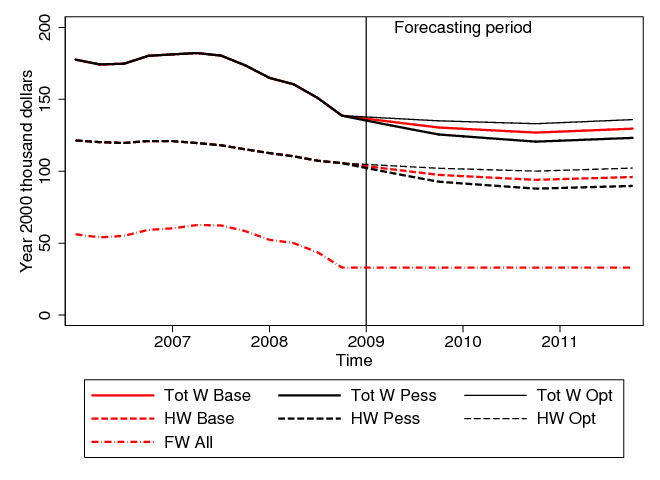
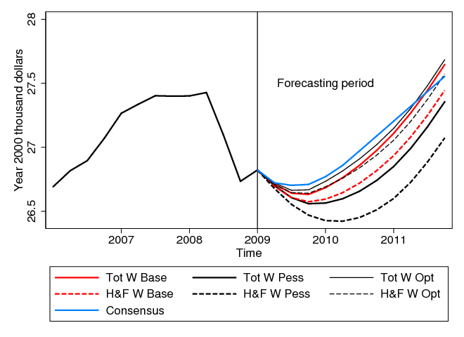
Figure 13 shows the projected consumption expenditure paths under the three
scenarios (of Table 3) and the two models—with total net worth, and
with wealth decomposed into separate housing and financial components
(Tables 1 and 2). We compare the six paths with the consumption
forecasts reported by Consensus Economics survey. Qualitatively, the
more pessimistic the scenario, the lower is consumption expenditure. In
addition, consumption projections of the disaggregated wealth model
(in which housing and financial wealth enter separately as independent
variables) are lower than those of the aggregate model because the estimated
MPC out of housing wealth is considerably larger than the MPC out of
financial wealth. Quantitatively, our models imply that per capita spending
will decrease from its current (2009Q4) level of $26,800 (in year 2000
dollars) by 0.6–1.5 percent before it starts to grow later this year or in
2010.
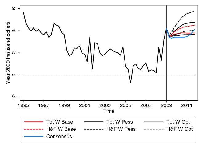
Figure 14 compares the saving rates with the benchmark saving rate implied by the Consensus
Economics survey.
Because of lower consumption paths our models generally predict higher saving
rates than the Consensus forecast. After the initial dip in 2009Q4 (caused by a
substantial fall in disposable income—3.5 percent in real per capita terms) the
saving rate typically tends to remain close to the current level of 4 percent but in
the most pessimistic scenario could increase to as much as 5.4 percent by the end
of 2011.
A more optimistic view is that the sluggishness in consumption growth in
historical data reflects the slow transmission of macroeconomic news to the
consumers’ consciousness; inattentive consumers are normally slow to react to
macroeconomic news because it takes them a while to notice it. This is the
optimistic interpretation of our empirical model’s results, because it would be
hard to argue that consumers have not noticed the current economic crisis.
Their adjustment may therefore have occurred much more quickly than
usual, so that the remaining degree of negative ‘momentum’ may be
negligible.
A further possibility worth mentioning is that spending on durable
goods may post sharp gains later this year; as Lawrence Summers has
pointed out, recent levels of automobile purchases are far below even the
level required merely to replace the stock that is depreciating due to
wear-and-tear or accidents. Indeed, a variety of measures from the recently
passed stimulus bill designed to encourage spending on durable goods
may make themselves felt later in the year and boost spending on those
categories.
But as noted above, the aggregate forecasting equation has tended to work
about as well for aggregate spending as for its components; we take this as
suggesting that spending on nondurable goods is likely to continue to be quite
weak even if durable goods spending recovers sharply. (In this case, one could
argue that consumers have indeed been ‘resting’ in their purchases of durable
goods).
Even if durables recover and nondurables stabilize in the near term, we are
inclined to believe that the end of the recent period of rapid credit expansion
portends a substantially higher saving rate two or three years hence than has
prevailed over the past few years. Returning to our remark in the introduction,
this would be the most favorable plausible scenario, because it would reflect a
path of Augustinian gradualism on the way to long-term reform. Such a
scenario would probably be the best outcome that can reasonably be hoped
for.
5 Conclusion
Since household spending has traditionally accounted for more than 2/3 of GDP,
consumer behavior always ends up being a decisive factor in macroeconomic
outcomes. But the degree of uncertainty about the spending outlook is
even greater now than usual. While our forecast is for slightly weaker
spending growth than called for by the Consensus survey of macroeconomic
forecasters, we would be remiss if we did not admit that the range of plausible
outcomes is very wide. No professional forecaster would be shocked if
the saving rate by the end of next year were as high as 8 percent (as
assumed in a pessimistic scenario in a recent report by Baily, Lund,
and Atkins (2009) of the McKinsey Global Institute) or as low as 2
percent.
Over the longer term, our best guess is that the gut-wrenching economic
uncertainty experienced in the current crisis will leave a lasting impression on
consumers’ attitudes toward debt; the combination of greater household
uncertainty and less adventurous credit supply by lenders, along with
households’ need to rebuild retirement and other wealth stocks devastated by the
crisis, will produce an eventual personal saving rate that is much higher than it
has been in many years.
References
BAILY, MARTIN N., SUSAN LUND, AND CHARLES ATKINS (2009): “Will US
Consumer Debt Reduction Cripple the Recovery?,” report, McKinsey Global Institute.
BOARD
OF GOVERNORS OF THE FEDERAL RESERVE SYSTEM (2009): “The Supervisory
Capital Assessment Program: Design and Implementation,” white paper, Available at
http://www.federalreserve.gov/newsevents/press/bcreg/20090424a.htm.
BOYD, DONALD J., AND LUCY DADAYAN (2009): “Sales Tax Decline
in Late 2008 Was the Worst in 50 Years,” State Revenue Report 75,
The Nelson A. Rockefeller Institute of Government, Available at
http://www.rockinst.org/pdf/government_finance/state_revenue_report/2009-04-14-(75)-state_revenue_report_sales_tax_decline.pdf.
CARROLL, CHRISTOPHER D. (2003): “Macroeconomic Expectations of Households
and Professional Forecasters,” Quarterly Journal of Economics, 118(1), 269–298,
Available at http://www.econ2.jhu.edu/people/ccarroll/epidemiologyQJE.pdf.
__________ (2009): “Lecture Notes: A Tractable
Model of Buffer Stock Saving,” Discussion paper, Johns Hopkins University, Available
at http://www.econ2.jhu.edu/people/ccarroll/public/lecturenotes/consumption.
CARROLL, CHRISTOPHER D., MISUZU OTSUKA, AND JIRKA SLACALEK (2009):
“How Large Are Housing and Financial Wealth Effects? A New Approach,”
Manuscript, Department of Economics, Johns Hopkins University, Available at
http://www.econ2.jhu.edu/people/ccarroll/papers/cosWealthEffects.
CARROLL, CHRISTOPHER D., MARTIN SOMMER, AND JIRI SLACALEK (2008):
“International Evidence on Sticky Consumption Growth,” Johns Hopkins University
Working Paper Number 542, Available at
http://www.econ2.jhu.edu/people/ccarroll/papers/cssIntlStickyC
http://www.econ2.jhu.edu/people/ccarroll/papers/cssIntlStickyC.pdf
http://www.econ2.jhu.edu/people/ccarroll/papers/cssIntlStickyC.zip.
DYNAN, KAREN E., AND DONALD L. KOHN (2007): “The Rise in U.S. Household
Indebtedness: Causes and Consequences,” International Finance Discussion Paper 37,
Board of Governors of the Federal Reserve System.
HALL, ROBERT E. (1978): “Stochastic Implications of the Life-Cycle/Permanent
Income Hypothesis: Theory and Evidence,” Journal of Political Economy, 96, 971–87,
Available at http://www.stanford.edu/~rehall/Stochastic-JPE-Dec-1978.pdf.
MIAN, ATIF, AND AMIR SUFI
(2008): “The Consequences of Mortgage Credit Expansion: Evidence from the 2007
Mortgage Default Crisis,” Forthcoming, Quarterly Journal of Economics, Available at
http://ideas.repec.org/p/nbr/nberwo/13936.html.


 Risk Rises
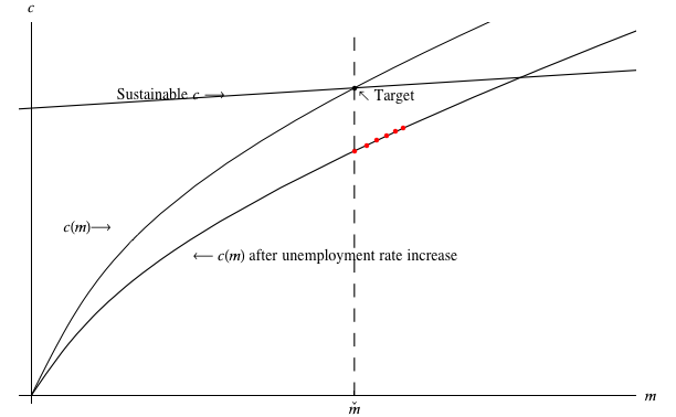
![∂CCCt+1 = ς + χ Et- 2[∂CCCt ] + ϵt+1 (1)](ReformingOrResting26x.png)